Introduction

My 2 month summer internship at Skymind (the company behind the open source deeplearning library DL4J) comes to an end and this is a post to summarize what I have been working on: Building a deep reinforcement learning library for DL4J: … (drums roll) … RL4J! This post begins by an introduction to reinforcement learning and is then followed by a detailed explanation of DQN (Deep Q-Network) for pixel inputs and is concluded by an RL4J example. I will assume from the reader some familiarity with neural networks. But first, lets talk about the core concepts of reinforcement learning.

Cartpole

Preliminaries

A “simple aspect of science” may be defined as one which, through good fortune, I happen to understand. (Isaac Asimov)

Reinforcement Learning is an exciting area of machine learning. It is basically the learning of an efficient strategy in a given environment. Informally, this is very similar to Pavlovian conditioning: you assign a reward for a given behavior and over time, the agents learn to reproduce that behavior in order to receive more rewards. It is an iterative trial and error process.

Markov Decision Process

Formally, an environment is defined as a Markov Decision Process (MDP). Behind this scary name is nothing else than the combination of (5-tuple):

• A set of states \(S\) (eg: in chess, a state is the board configuration)
• A set of possible actions \(A\) (In chess, all the move that could be possible in every configuration possible, eg: e4-e5)
• The conditional distribution \(P(s'| s, a)\) of next states given a current state and an action. (In a deterministic environment like chess, transitioning from state \(s\) with action \(a\), there is only one state s’ with probability 1, and all the others have probability 0. Nevertheless, in a stochastic (involving randomness, eg: a coin toss) environment, the distribution is not as simple.)
• The reward function of transitionning from state s to s’: \(R(s, s')\) (eg: In chess, +1 for a final move that leads to a victory, -1 for a final move that leads to a defeat, 0 otherwise. In Cartpole, +1 for each step.).
• The discount factor: \(\gamma\). This is the preference for present rewards compared to future rewards. (A concept very common in finance.)

Note: It is usually more convenient to use the set of Action \(A_s\) which is the set of available move from a given state, than the complete set A. \(A_s\) is simply the elements \(a\) in \(A\) such that \(P(s' | s, a) > 0\).

The markov property is to be memoryless. Once you reach a state, the past history (the states visited before) should not affect the next transitions and rewards. Only the present state matters.

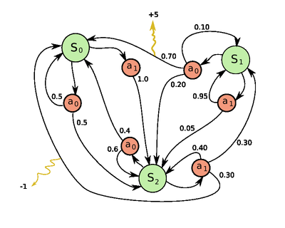
Schema of a MDP

Some terminologies

Final/terminal states: The states that have no available actions are final/terminal states.

Episode: An episode is a complete play from one of the initial state to a final state. \[s_0, a_0, r_0, s_1, a_1, r_1, \ldots, s_n\]

Cumulative reward: The cumulative reward is the discounted sum of reward accumulated throughout an episode: \[R=\sum_{t=0}^n \gamma^t r_{t+1}\]

Policy: A Policy is the agent’s strategy to choose an action at each state. It is noted by \(\pi\).

Optimal policy: The optimal policy is the theoretical policy that maximizes the expectation of cumulative reward. From the definition of expectation and the law of large numbers, this policy has the highest average cumulative rewards given sufficient episode. This policy might be intractable.

The objective of reinforcement learning is to train an agent such that his policy converges to the theoretical optimal policy.

Different settings

« Qui peut le plus peut le moins » (He who can do the greater things, can do the lesser things)

Model-free

The conditional distribution and the reward function constitute the model of the environment. In a game of backgammon, we know the model (each possible transition is decided by the known dice distribution, and we can predict each reward from transition without realizing them (because we can calculate the new value of the board)). The algorithm TD-gammon use that fact to learn the V-function (see below).

Some reinforcement learning algorithms can work without being given the model. Nevertheless, in order to learn the best strategy, they additionaly have to learn the model during the training. This is called model-free reinforcement learning. Model-free algorithms are very important because a large majority of real world complex problems fall in that category. Futhermore, model free is simply an additional constraint. It is simply more powerful since it is a superset of model based reinforcement learning.

Observation setting

Instead of being given access to the state, you might being given access to a partial observation of the state only. It is the same idea behind Hidden Markov Chain. This is the difference between the partial and fully observed setting. For instance, our field of vision is a very partial observation of the full state of the universe (the position and energy of every particule in the universe). Fortunately, the partial observation setting can be reduced to a fully observed setting with the use a history (the state becomes an accumulation of previous states).

Nevertheless, it is most common to not accumulate the whole history. Either only the last h observations are stacked (in a windowed fashion) or you can use a Recurrent Neural Network (RNN) to learn what to keep in memory and what to forget (that is essentially how a LSTM works).

Abusing the language slighty for consistency purposes with the existing notation, history (even truncated ones) will also be called “state” and also symbolized \(S_t\)

Single player and adversarial games

A single player game has a natural translation into a MDP. The states represent the moment where the player is in control. The observations from those states are all the information accumulated between states (eg: as many pixel frame as there are in-between frames of control). An action is all the available command at the disposal of the player (In doom, go up, right, left, shoot, etc …).

Reinforcement learning can also be applied to adversarial games by self-play: The agent plays against itself. Often in this setting, there exists a Nash equilibrium such that it is always in your interest to play as if your opponent was a perfect player. This makes sense in chess by example. If given a board configuration, a good move against a chess master, would still be a good move against a beginner.¹ Whatever is the current level of the agent, by playing against himself, the agent stills get information about the quality of his previous moves (seen as good moves if he won, bad moves if he lost).

Of course the information, which is a gradient in the context of a neural network, is of «higher quality» if he played directly against a very good agent from the start. But it is really mind-blowing that an agent can learn to increase his level of play by playing against himself, an agent of the same level. That is actually the method of training employed by AlphaGo (the Go agent from DeepMind that beat the World Champion). The policy was bootstrapped (initially trained) on a dataset of master moves, then it used reinforcement learning and self play to increase furthermore the level (quantified with elo). In the end, the agent got better than policy it was learning from the original dataset. After all, it beat the master above all the masters. To compute the final policy, they used their policy gradient in combination with a Monte-Carlo Search Tree on a massive amount of computation power.

This setting is a bit different from learning from pixels. Firstly, because the input is not as high-dimensional. The manifold is a lot closer to its embedding space. Nevertheless, a convolutional layer was still used in this case to use efficiently the locality of some subgrid board patterns. Secondly, because AlphaGo is not model-free (it is deterministic). In the following of this post, I will talk exclusively about the model-free 1-player setting.

Q-learning

I am no friend of probability theory, I have hated it from the first moment when our dear friend Max Born gave it birth. For it could be seen how easy and simple it made everything, in principle, everything ironed and the true problems concealed. (Erwin Schrödinger)

From policy to neural network

Our goal is to learn the optimal policy \(\pi^*\) that maximize: \[E[R_0]=E[\sum_{t=0}^n \gamma^t r_{t+1}]\] Let’s introduce an auxilliary function: \[V_\pi(s) = E \{ r_t + \gamma r_{t+1} + \gamma^2 r_{t+2} + \ldots + \gamma^n r_{n} \mid s_t = s, \text{policy followed at each state is }\pi \}\] which is the expected cumulative reward from a state \(s\) following the policy \(\pi\). Let suppose an oracle \[V_{\pi^*}(s)\] The V function of the optimal policy. From it, we could retrieve the optimal policy by defining the policy that among all available actions at the current state, choose the action that maximize the expectation of \(V_{\pi^*}(s)\). This is a greedy behavior. The optimal policy is the greedy policy w.r.t to \(V_{\pi^*}\). \[ \pi^*(s) ~\text{chooses a s.t}~a= arg \max_a[E_\pi(r_t + \gamma V(s_{t+1}) \mid s_t=s, a_t=a)] \] If you were very attentive, something would sound wrong here. In the model-free setting, we cannot predict the after-state \(s_{t+1}\) from \(s_{t}\) because we ignore the transition model. Even with that oracle, our model is still not computable!

To solve this very annoying issue, we are gonna use another auxiliarry function, the Q-function: \[Q_{\pi^*}(s, a) = E_\pi[r_t + \gamma V_{\pi^*}(s_{t+1}) \mid s_t, a_t = a]\] In a greedy setting, we have the relationship: \[V_\pi(s_t) = \max_a Q_\pi(s_t, a)\] Now, let suppose instead of the V oracle, we have the Q oracle. We can now redefine \(\pi^*\). \[ \pi^*(s) ~ \text{chooses a s.t}~ a= arg \max_a[Q_{\pi^*}(s, a)] \] No more uncomputable expectations, Neat

Nevertheless, we have only moved the expectation from outside to inside the oracle. And unfortunately, oracles do not exist in the real world.

The trick here is that we have reduced an abstract notion that is a policy into a numerical function that might be relatively “smooth” (continuous) thanks to the expectation. Fortunately for us, there is one weapon at our disposal to approximate such complex functions: Neural networks.

Neural networks are universal function approximators. They can approximate any continuous differentiable function. Although they can get stuck in local extrema and many proofs of convergence from reinforcement learning are not valid anymore when throwing neural networks in the equation. This is because their learning is not as deterministic or boundable as their tabular counterparts. Nonetheless, in most case, with the right hyperparameters, they are unreasonnably powerful. Using deep learning with reinforcement learning is called deep reinforcement learning.

Policy iteration

Now machine learning knowledge and common sense tells you that there is still something missing about our approach. Neural networks can approximate functions that already have labels. Unfortunately for us oracles are not summonable, so we will have to get our labels another way. (:<).

This is where the magic of Monte Carlo come in. Monte carlo methods are methods that rely on repeated random sampling to calculate an estimator. (A famous example is the pi calculation).

If we play randomly from a given state, the better states should get better rewards on average (thank you law of large numbers). So without knowing anything about the environment, you can get some information about the expected value of a state. For instance, at poker, better hands will win more often on average than lesser hands even when every decision is taken randomly. The Monte Carlo Search Tree are also based on this property (shocking isn’t it?). This is a phase of exploration that lead to unsupervised learning and enable us to extract meaningful label.

More formally,

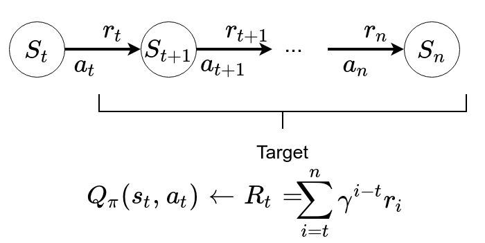
Given a policy \(\pi\), a state s and an action a, in order to get an approximation of \(Q(s, a)\) we sample it according to its definition:

In plain english, we can get a label for \(Q_\pi(s, a)\) by playing a sufficient number of time from s according to the policy \(\pi\).

From an aggregate of signals:

One signal

The actual learning is done by standard Gradient descent, using the labels in batches. The gradient is the standard Mean-Square Error one such that the td-error gets minimised at each iteration.

We use the Mean-Square Error loss function (l2 loss) with a learning rate of \(\alpha\) and apply Stochastic Gradient Descent (On a batch of size 1) of: \[Q_\pi(s_t, a_t) \leftarrow Q_\pi(s_t, a_t) + \alpha [R_t-Q_\pi(s_t, a_t)]\]

\((s_t, a_t)\) is the input, \(Q_\pi(s_t, a_t) + \alpha [R_t-Q_\pi(s_t, a_t)]\) is the label aka target.

Note: Even if we use MSE, there is no square in the formula because the loss is applied afterwards on the difference of the expected output \(Q_\pi(s_t, a_t)\) and the label \(\alpha [R_t-Q_\pi(s_t, a_t)]\).

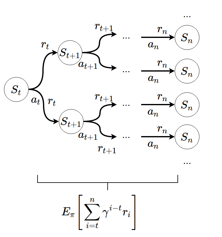
Repeat many times: Sampling from \(\pi\) \[Q_\pi(s_t, a_t) \leftarrow E_\pi[R_t] = E_{s_t, a_t, ..., s_n \sim \pi}[\sum_{i=t}^n \gamma^{i-t}r_i]\] We can converge to the rightful expectation

Many signals

So we can now design a naive prototype of our learning algorithm (in Scala but it is intelligible without any Scala knowledge):

//A randomly uninitialized neural network
val neuralNet: NeuralNet

//Iterate until you reach max epoch
for (t <- (1 to MaxEpoch))
	epoch()


def epoch() = {

	//pick a random state and action
	val state = randomState
	val action = randomAction(state)

	//transition to a new state, initalize thethe reward
	var (new_state, accuReward) = transitition(state, action)

	//play until terminal state and accumulate the reward
	accuReward += playRandomly(state)

	//Do SGD over input and label!
	fit((state, action), accuReward)
}



// MDP specific, return the new state and the reward
def transition(state: State, action: Action): (State, Double)

//return a randomly sampled state among all the state space
def randomState: State

//play until terminal state
def playRandomly(state): Double = {
	var s = state
	var accuReward = 0
	var k = 0
	while (!s.isTerminal) {
		val action = randomAction(s)
		val (state, reward) = transition(s, action)
		accuReward += Math.pow(gamma, k) * reward
		k += 1
		s = state
	}
	accuReward
}


//choose a random action among all the available actions at this state
def randomAction(state: State): Action =
	oneOf(state.available_action)

//helper function, pick one among
def oneOf(seq: Seq[Action]): Action =
	seq.get(Random.nextInt(seq.size))


//How it would be roughly done with DL4J
def fit(input: (State, Action), label: Double) =
	neuralNet.fit(toTensor(input), toTensor(label))

//return an INDArray from ND4J
def toTensor(array: Array[_]): Tensor =
	Nd4j.create(array)

There are multipqle issues: This should work but this is terribly inefficient. We are playing a full game with n state and n actions for a single label and that label might not be very meaningful (If the interesting trajectories are hard to reach at random).

The Exploration/Exploitation dilemma

Exploring at random the environment will converge to the optimal policy … but only guaranteed after an almost infinite time: you will have to visit every possible trajectories (a trajectory is the ordered list of al the states visited and actions choosen during an episode) at least once. Considering how many states and branching there is, it is impossible. The branching issue is the reason why Go is so hard but chess is ok. In the real world, we do not have infinite time (and time is money).

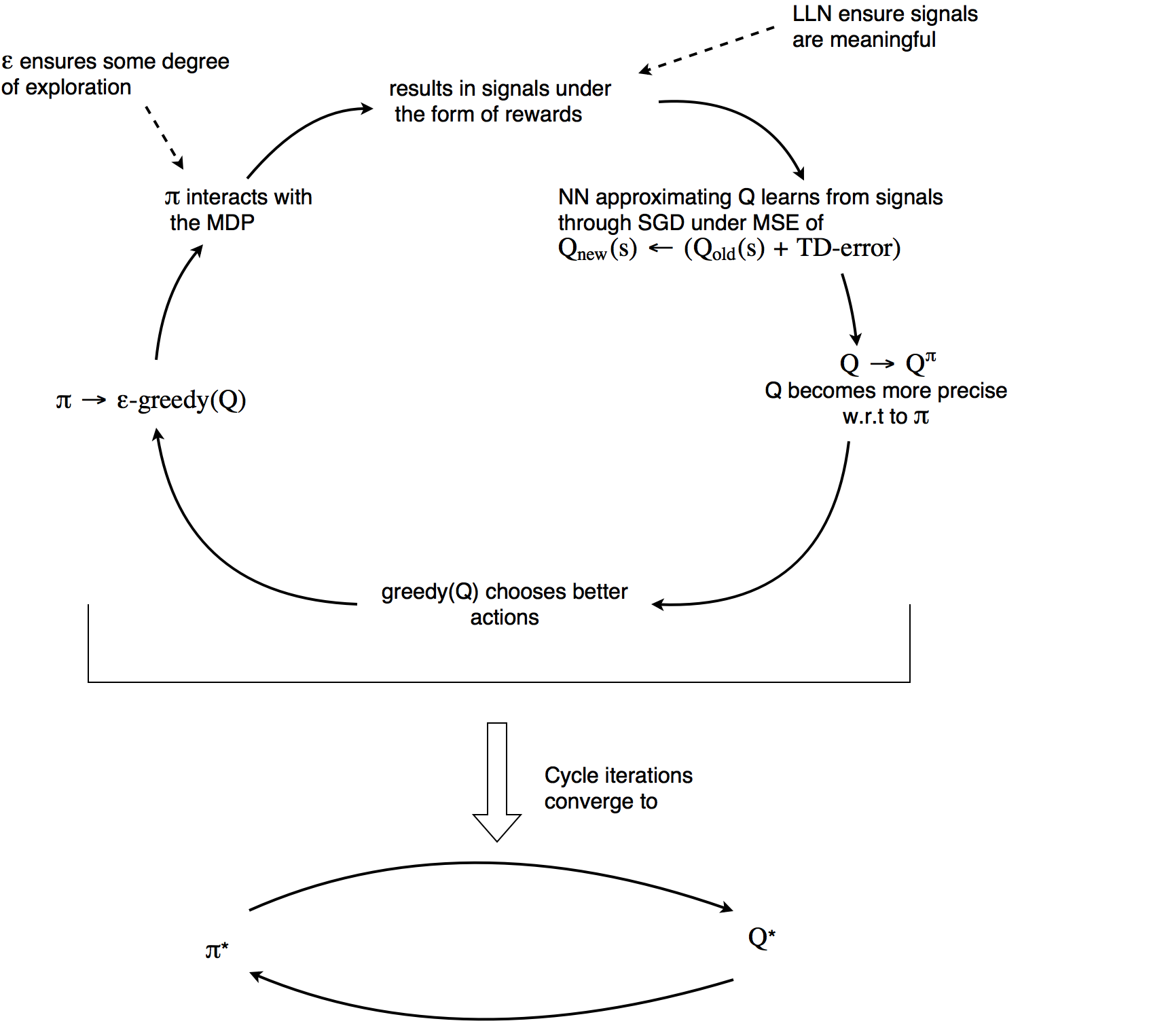
Thus, we should exploit the past informations and our learning of them to focus our exploration on the most promising possible trajectories. This can be achieved through different ways, and one of them is \(\epsilon\)-greedy exploration. \(\epsilon\)-greedy exploration is fairly simple. It is a policy that choose an action at random with odd \(\epsilon\) or the best action as deemed by our current policy with odd \((1-\epsilon)\). Usually \(\epsilon\) is annealed over time to privilege exploitation over exploration after enough exploration. This is a trade-off between exploration and exploitation.

At each new information, our actual Q functions gets more accurate about the present policy and the exploration is focused on better paths. The policy based on our new Q function gets better (since Q is more accurate) and the \(\epsilon\)-greedy exploration reach better paths. Focused on those better paths, our q function explore even more the better parts and has to update its returns according to the new policy. This is an iterative cycle that enable convergence to the optimal policy called policy iteration. Unfortunately, the convergence can take infinite time and is not even guaranteed when Q is approximated by neural networks. Nevertheless, impressive results can make up for the lack of formal convergence proofs.

Policy Iteration

This algorithm also requires you to be able to sample the states in a «good» manner: It should be proportionally representative of the states that are usally present in a game (or at least the kind of game at the targeted agent’s level). On a sidenote, this is possible in some case, see Giraffe that uses TD-Lambda.

Fortunately, some rearranging and optimisations are possible:

Bellman equation

As in the Monte-Carlo method, we can do many updates of Q.

MSE: \[Q_\pi(s_t, a_t) \leftarrow Q_\pi(s_t, a_t) + \alpha [(\underbrace{\underbrace{r_t+\max_a Q_\pi(s_{t+1}, a)}_{\text{target}}-Q_\pi(s_t, a_t)}_{\text{TD-error}})]\]

TD-error is the “Temporal difference error”. Indeed, we are actually calculating the difference between what the Q approximation expects in the future plus the realized reward and its present value as evaluated by the neural net.

That bellman equation only make sense with some boundary conditions. if s is terminal: \[V(s) = 0\] and for any a \[Q(s_{t-1}, a) = r_t\]

The states near the terminal states are the first to converge because they are closer in the chain to the «true» label, the known boundary conditions. In Go or Chess, reinforcement learning is applied by assigning +1 to the transitions that lead to a final winning board (respectively -1 for a loosing board) and 0 otherwise. It diffuses the Q-values by finding a point between the two extremes [-1; 1]. A transition with Q value close to 0 represents a transition leading to a balanced board. A transition with Q value close to 1 represents a near certain victory.

It could be surprising that the moves do not have only -1 and 1 values (since deviating from the optimal path should be fatal). One interesting aspect of calculating Q-values is the realization that in many games/MDP, no mistake in itself is ever really fatal. It is the accumulation of them that really kill you. AI is full of life lessons ;). Moreover, The expected accumulated reward space is a lot smoother than often thought. One possible explanation is that expectations always have an average effect: an expectation is nothing else than a weighted average with probabilities as weights. Furthermore, gamma being \(< 1\) the very long-term effects are not too preponderant. Isn’t it exciting to be able to calculate directly the odd of winning a game for every transition ?

As long as we sample sufficiently enough transitions near the terminal states, Q-learning is able to converge. The incredible power of deep reinforcement learning is that it will be able to generalize its learning from visited states to unvisited states. It should be able to understand what is a balanced or winning board even if it has never seen it before. This is because the network should be able to abstract patterns and understand the strength of an action based on previously seen pattern (eg: shoot an enemy when recognizing its form).

Offline and online reinforcement learning

To learn more about the differences between online and offline reinforcement learning, see this excellent post from kofzor.

Initial state sampling

In a 1 player setting (like the atari game): We do not actually need to learn to play well in every situation (Although, if we did, that would show that we would have reached a very good level of generalization). We only need to learn to play efficiently from the states that our policy encounters. Thus, we can sample from states that are simply reachable by playing with our current policy from an initial state. This enables to sample directly from a played episode by our agent.

Q-Learning implementation

So we can now design a naive prototype of our Q-Learning:

def epoch() = {

	//sample among the initial state space
	//(often unique state)
	var state = initState

	//while the state is not terminal,
	//play an episode and do a Q-update at each transition
	while(!state.isTerminal)  {

		//sample action from eps-greddy policy
		val action = epsilonGreedyAction(state)

		//interaction with the environment
   		val (nextState, reward) = transition(state, action)

		//Q-update
		update(state, action, reward, nextState)

		state = nextState
	}
}

//Our Q-update as explained above
def update(state: State, action: Action, reward: Double, nextState: State) = {
	val target = reward + maxQ(nextState)
	fit((state, action), target)
}


//the eps-greedy policy implementation
def epsilonGreedyAction(state: State) = {
	if (Random.float() < epsilon)
		randomAction(state)
	else
		maxQAction(state)
}


//Retrive max Q value
def maxQ(state: State) =
	actionsWithQ(state).maxBy(_._2)._2

//Retrive action of the max Q value
def maxQAction(state: State) =
	actionsWithQ(state).maxBy(_._2)._1

//return a list of actions and the q-value of their transition from the state
def actionsWithQ(state: State) = {
	val stateActionList = available_actions.map(action => (state, action))
   	available_actions.zip(neural_net.output(toTensor(state_action_list)))

def initState: State

Modeling Q(s, a)

Instead of having \(a\) as an additional input of the neural net combined with the state, the state is the only input and the output contains the Q value of every action possible. This makes sense only when the availables actions are consistent accross the full episode (else the neural output layer would have to be different at each state). It is many times solvable by having the full set \(A\) of actions as output and ignore the impossible actions (some papers put the target of impossible actions at 0).

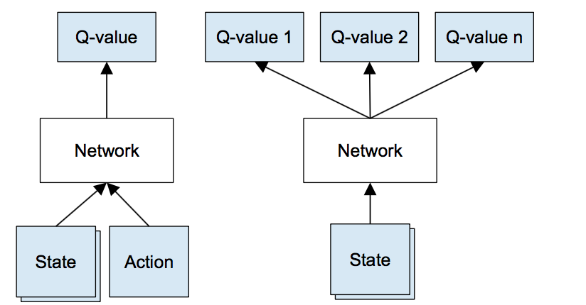
Q modeling Source

Experience replay

There is one issue with using neural network as Q approximator. The transitions are very correlated. This reduce the overall variance of the transition. After all, they are all extracted from the same episode. Imagine if you had to learn a task without any memory (not even short-term), you would always optimise your learning based on the last episode.

The Google DeepMind research team used experience replay, which is a windowed buffer of the last N transitions (N being a million in the original paper) with DQN and greatly improved their performances on atari. Instead of updating from the last transition, you store it inside the experience replay and update from a batch of randomly sampled transitions from the same experience replay.

epoch() becomes:

def epoch() = {

	//sample among the initial state space
	//(often unique state)
	var state = initState

	//while the state is not terminal,
	//play an episode and do a Q-update at each transition
	while(!state.isTerminal)  {

		//sample action from eps-greddy policy
		val action = epsilonGreedyAction(state)

		//interaction with the environment
   		val (nextState, reward) = transition(state, action)

		//store transition (Exp Replay is just a Ring buffer)
		expReplay.store(state, action, reward, nextState)

		//Q update in batch
		updateFromBatch(expReplay.getBatch())

		state = nextState
	}
}

Compression

nd4j, the tensor library of dl4j, does not support as first class type uint8. However, pixels in grayscaling are encoded with that precision. To avoid wasting too much space on memory, INDArray were compressed to uint8.

Convolutional layers and image preprocessing

Convolutional layers

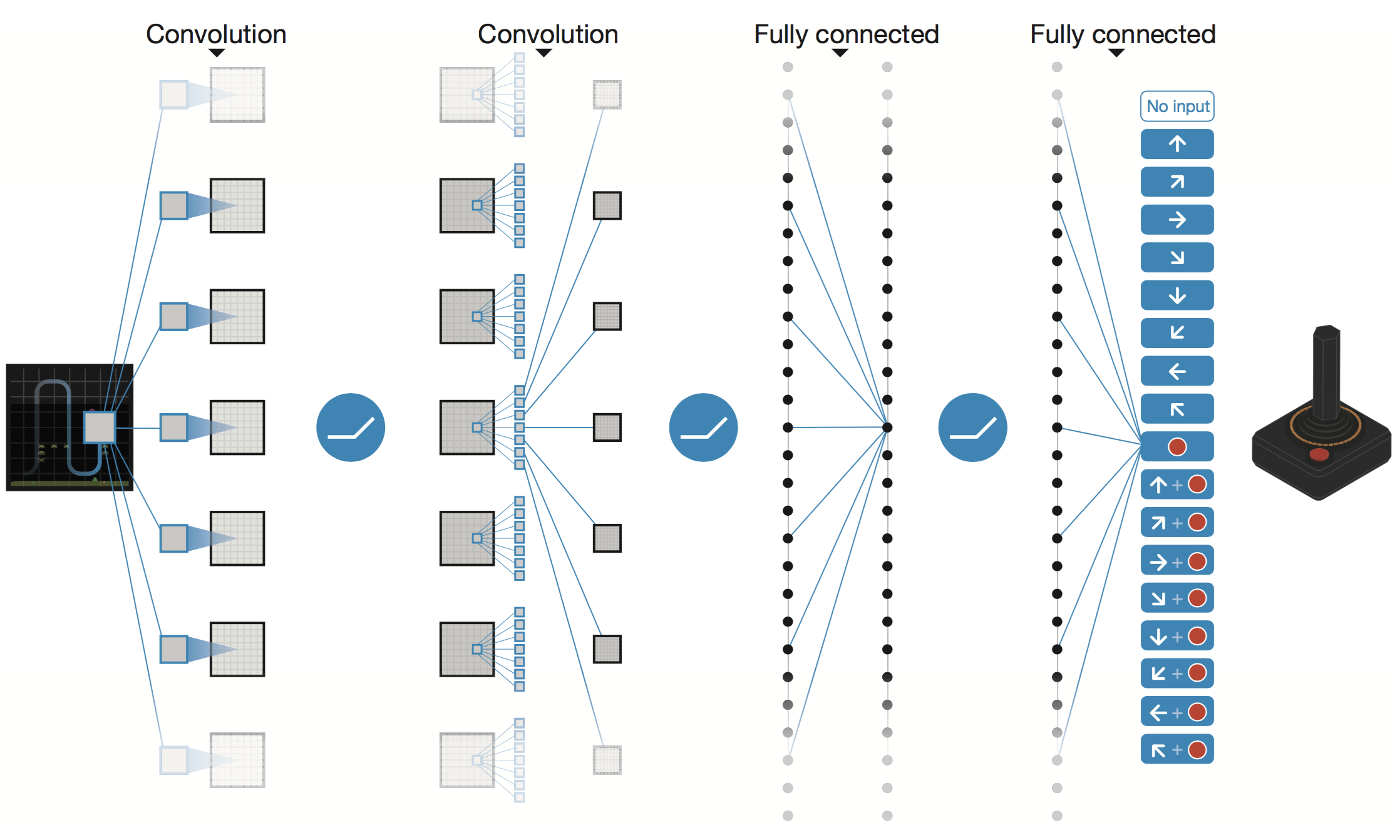
Convolutional layer Source

Convolutional layers are layers that are excellent to detect local patterns in images. For pixels, it is used as a processor that is required to reduce the dimension of the input into its real manifold. Given the proper manifold of observations, the decision becomes much easier.

Image processing

You could feed the neural network with the RGB directly, but then the network would have to also learn that additional pattern. It seems like the brain is hard-wired to combine colors (fortunately!). Thus, it would seem reasonnable to tolerate that preprocessing.

What you see:

What the neural net see:

Neural net input

resizing

The image is resized into 84x84. Convolutional layers needs for memory and computations grow with the size of their input. The fine details of the image are not required to play the game correctly. Indeed, many are purely aesthetic. Resizing to a more reasonnable size speed up the training.

Skip frame

In the original atari paper, only 1 in 4 frames is actually processed. For the following 3 images, the last action is repeated. It speeds up roughly by 4 time the training without loosing much information. Indeed, atari game are not supposed to be played frame perfect and for most action it makes more sense to keep them for at least 4 frames.

History Processing

To give information to the Neural network about the current momentum, the last 4 frame (with skip frame, you pick 1 every 4) are stacked into 4 channels. Those 4 frames represent a history as previously discussed in the Observation setting section.

Slowed input

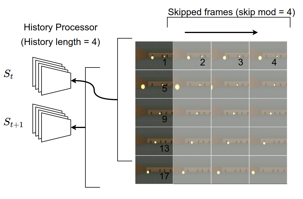
Stacking

To fill the first frames of the history, a random policy or a noop replay is used. (Sidenote, random starts can be used for fair evaluation)

Double Q-learning

The idea behind double DQN is that the network is frozen every M update (hard update) or smoothly averaged (target = target * (smooth) + current * (1-smooth)) every update (soft update). Indeed, it adds stability to the learning by using a Q evaluation to use in the td-error formula that is less prone to “jiggering”. The Q update becomes:

\[Y_\text{target} = r_t + \gamma*(Q_\text{target}(s_t+1, arg \max_a Q_\text(s_t+1, a))) \]

Clipping

The TD-error can be clipped (bounded between two limit values) such that no outlier update can have too much impact on the learning.

Scaling rewards

Scaling the rewards such that Q-values are lower (in a range of [-1; 1] is similar to normalization). It can dramatically alter the efficiency of the learning. This is an important hyperparameter to not neglect.

Prioritized replay

The idea behind prioritized replay is that not all transitions are born equal. Some are more important than others. One way to sort them is through their TD-error. Indeed, a high TD-error is correlated to a high level of information (in the sense of surprise). Those transitions should be sampled more often than the others.

Graph, Visualisation and Mean-Q

To visualize and debug the training or a method of RL, it is useful to have a visual monitoring of the agent’s progress. This is why I built the dashboard webapp-rl4j.

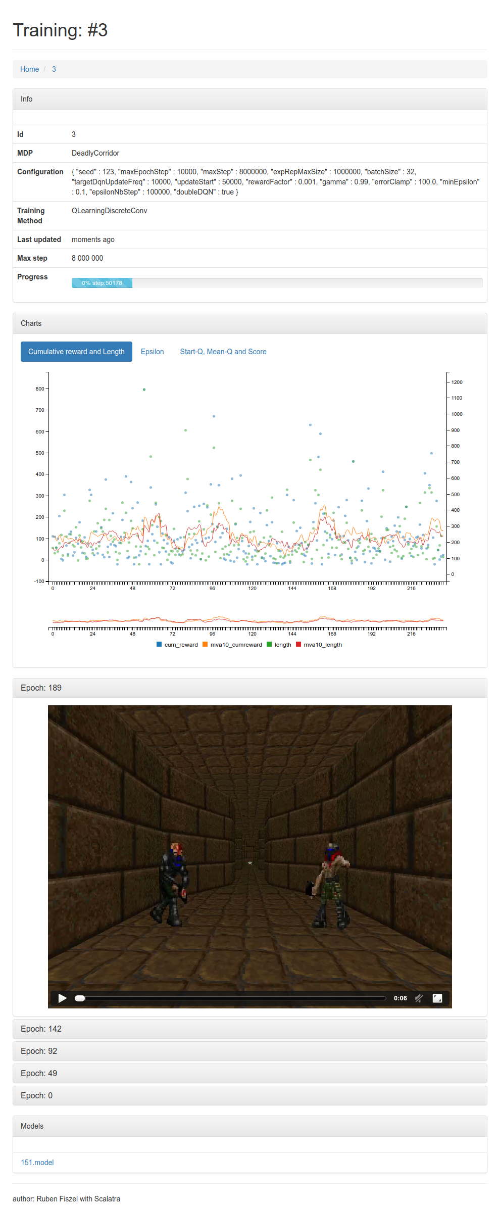
webapp-rl4j

The most important is to keep track of cumulative rewards. This is a way to check that the agents effectively gets better. It is important to notice that it represents the epsilon greedy strategy and not the directly derived policy from the Q approximation.

Cumulative reward graph

But you might want to also track the loss (score of the neural network) and mean Q-values:

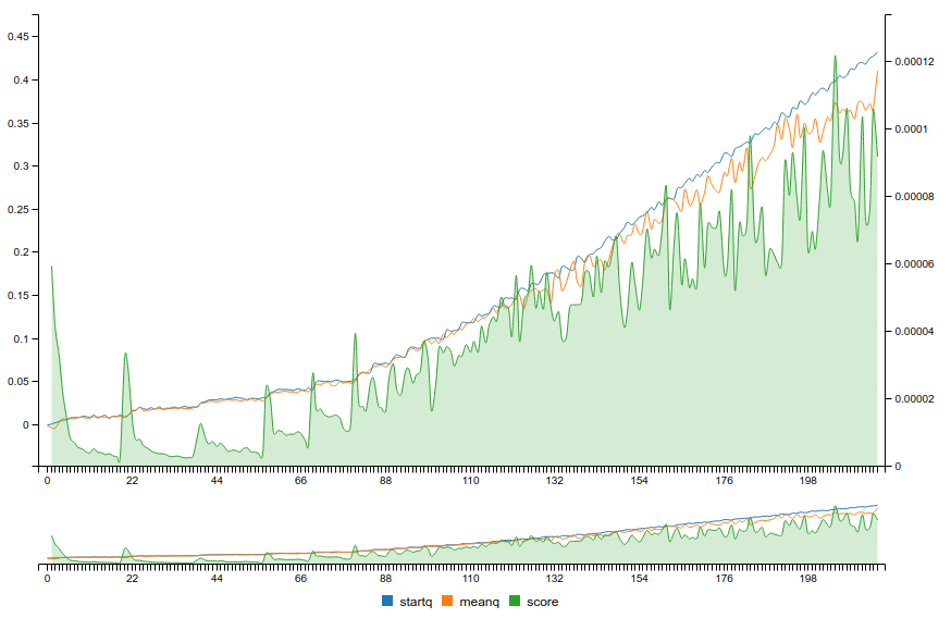
Score and mean-Q graph

Unlike with classic supervised learning, the loss does not necessarily always decrease because the learning impacts the labels!

If used with target network, you should see some discontinuities from the non continuous evaluation of different target networks. Loss should decrease w.r.t to a single target network. The mean Q-values should smoothly converge towards a value proportionnal to the mean expected reward.

RL4J

RL4J is available on github. Currently DQN with Experience Replay, Double Q-learning and clipping is implemented. Asynchronous Reinforcement Learning with A3C and Async N-step Q-Learning is included too. It is possible to play both from pixels or low-dimensional problems (like Cartpole). Async Reinforcement Learning is experimental. Hopefully, contributions will enrich the library.

Here is a working example with RL4J to play Cartpole with a simple DQN. You can play Doom too. Check rl4j-examples for more examples. It is also possible to provide your own constructed neural network model as an argument to any training method.

    public static QLearning.QLConfiguration CARTPOLE_QL =
            new QLearning.QLConfiguration(
                    123,    //Random seed
                    200,    //Max step By epoch
                    150000, //Max step
                    150000, //Max size of experience replay
                    32,     //size of batches
                    500,    //target update (hard)
                    10,     //num step noop warmup
                    0.01,   //reward scaling
                    0.99,   //gamma
                    1.0,    //td-error clipping
                    0.1f,   //min epsilon
                    1000,   //num step for eps greedy anneal
                    true    //double DQN
            );

    public static DQNFactoryStdDense.Configuration CARTPOLE_NET =
            new DQNFactoryStdDense.Configuration(
                    3,         //number of layers
                    16,        //number of hidden nodes
                    0.001,     //learning rate
                    0.00       //l2 regularization
            );

    public static void main( String[] args )
    {

        //record the training data in rl4j-data in a new folder (save)
        DataManager manager = new DataManager(true);

        //define the mdp from gym (name, render)
        GymEnv<Box, Integer, DiscreteSpace> mdp = new GymEnv("CartPole-v0", false, false);

        //define the training
        QLearningDiscreteDense<Box> dql = new QLearningDiscreteDense(mdp, CARTPOLE_NET, CARTPOLE_QL, manager);

        //train
        dql.train();

        //get the final policy
        DQNPolicy<Box> pol = dql.getPolicy();

        //serialize and save (serialization showcase, but not required)
        pol.save("/tmp/pol1");

        //close the mdp (close http)
        mdp.close();


    }

Conclusion

This was an exciting journey through deep reinforcement learning. From equations to code, Q-learning is a powerful, yet a somewhat simple algorithm. The field of RL is very active and promising. In fact, Supervised learning could be considered a subset of Reinforcement learning (by setting the labels as rewards). Maybe one day, Reinforcement Learning will be the panacea of AI. Until then, we can expect to be awed by its diverse applications into more and more mind-blowing problems. As a word of acknowledgement, I would like to thank Skymind and its amazing team for this very enriching internship.

To feed your appetite

Bookworm

I hope that thanks to this introduction, you are excited about RL research. Here is a brief summary of important research in deep reinforcement learning.

Continuous domain

When the action space is not discrete, you cannot use DQN. But many problems cannot be discretized. Continuous control is achieved through a normal distribution parametrized (mean and variance) by the output of the neural network. At each step, the action is sampled from the distribution. It also uses soft update of the target network.

Policy gradient

Policy gradient works by directly learning the stochastic policy from cross entropy of the distribution scaled bythe advantage. This excellent post from Karpathy’s blog has more details on the matter. Using a stochastic policy feels more natural as it encourages exploration and exploit more fairly the uncertainty we have between the different values of the move. Indeed, a max operation can end by ignoring fully a branch that is \(\epsilon\) below in Q-value of another. Although, This can be solved in DQN by using Boltzmann exploration.

Policy gradient were used by AlphaGo in combination with MonteCarlo Search Tree. The Neural Network was bootstrapped (pretrained) on a dataset of master move before they let it improve itself with RL.

Nowadays, policy gradients are getting more popular. For example, A3C (see below) is based on it.

Asynchronous Methods for Deep Reinforcement Learning

A3C (Asynchronous Actor Critic) and Async NStep Q learning are included in RL4J. It bypasses the need for an experience replay by using multiple agents exploring in parrallel the environment. The original paper uses Hogwild!. In RL4J, a workaround is to use a central thread and accumulate gradient from “slave” agents. Having multiple agents exploring the environment enable to decorrelate the experience from the past episode and enable to gather more experience (instead of replaying multiple time the same transition). It is very efficient and the authors were able to train efficiently on a single machine!

For the curious, here is some Scala-pseudo-code of A3C:

//A randomly uninitialized neural network
val globalNeuralNet: NeuralNet

//Iterate until you reach max epoch
for (t <- (1 to numThread))
	launchThread()

def launchActor) =
  new Actor(globalNeuralNet).run()

var globalT: Int = 0

class Actor(globalNeuralNet: NeuralNet) {

  def run() = {
    while(globalT < maxStep) {

      val neuralNet = globalNeuralNet.clone()

      var state = initState
      var i = 0
      val stack:Stack[(State, Action, Reward)] = new Stack()

      while(i < tMax && !state.isTerminal){
        globalT += 1
        i += 1

	//sample action from stochastic policy
	val action = stochasticPolicy(neuralNet, state)

	//interaction with the environment
   	val (nextState, reward) = transition(state, action)
        stack.add((state, action, reward))
        state = nextState

      }

      var r =
        if (state.isTerminal)
          0
        else
          criticOutput(neuralNet, state)

      val inputs = new Tensor()
      val actorLabels = new Tensor()
      val criticLabels = new Tensor()

      while(!stack.isEmpty) {
        val trans = stack.dequeue()
        r = trans.reward + gamma*r

        inputs.appendRow(trans.state)
        criticLabels.appendRow(r)

        val prevCriticOutput = criticOutput(neuralNet, trans.state)
        val advantage = r - prevCriticOutput
        val prevActorOutput = actorOutput(neuralNet, trans.state)

        actorLabel.appendRow(prevActorOutput.addScalar(trans.action, r))

      }

      asyncUpdate(globalNeuralNet, inputs, criticLabels, actorLabels)

    }
  }

  def stochasticPolicy(neuralNet: NeuralNet, state: State) = {
    val distribution = actorOutput(neuralNet, state)
    chooseAccordingToDistribution(state.availableActions, distribution)
  }


}

Deep exploration

Deep exploration was the subject of a semester project during my master. I wrote the Scala library scala-drl about it. Deep exploration is defined as the multi-step ahead planning of the exploration.

In Bootstrapped DQN, the term bootstrapping comes from statistics. Multiple neural network are constructured in parralel. At each epoch, one neural network explore the environment. Then the transition are randomly redistributed to each model. This has a similar effect than resampling. Having had differences experiences to learn from, each model has its own opinion about the best move and its own uncertainty about the environment. This encourage deep exploration.

Another way is to use Autoencoder to quantify the uncertainty about a novel state and attribute an exploration bonus based on the reconstruction loss.

Other interesting papers to discover by yourself.

Deterministic Policy Gradient

http://jmlr.org/proceedings/papers/v32/silver14.pdf

Trusted Region Policy Optimisation

https://arxiv.org/abs/1502.05477

Dueling Network Architectures for Deep Reinforcement Learning

http://arxiv.org/abs/1511.06581

References

Karpathy’s post about Policy Gradient

Playing Atari with Deep Reinforcement Learning

Deep Reinforcement Learning with Double Q-learning

Asynchronous Methods for Deep Reinforcement Learning

Prioritized Experience Replay

Continuous control with deep reinforcement learning

Giraffe: Using Deep Reinforcement Learning to Play Chess

Deep Exploration via Bootstrapped DQN

Incentivizing Exploration In Reinforcement Learning With Deep Predictive Models

REINFORCEjs

Sutton holy bible on reinforcement learning