(thesis 2/4) A simulation tool for scala with spatial integration: scala-flow

Posted on August 16, 2017 by Ruben Fiszel

About

This post is the part II out of IV of my master thesis at the DAWN lab, Stanford, under Prof. Kunle and Prof. Odersky supervision. The central themes of this thesis are sensor fusion and spatial, an hardware description language (Verilog is also one, but tedious).

This part is about scala-flow, a simulation library with a spatial-lang integration written to ease the prototyping, development and testing of applications that can be represented as data flows with some subpart going through spatial written accelerators.

A simulation tool for data flows with Spatial integration: scala-flow

Purpose

Data flows are intuitive visual representations and abstractions of computation. As all forms of representations and abstractions, they ease complexity management, and let engineers reason at a higher level. They are common in the context of embedded systems, where sensors and electronic circuits have natural visual representations. They are also used in most forms of data processing, in particular those related to so called big data.

Spark and Simulink are popular libraries for data processing and embedded systems, respectively. Spark grew popular as an alternative to Hadoop. The advantages of Spark over Hadoop was, among others, in-memory communication between nodes (as opposed to through files) and a functionally inspired scala api that brought better abstractions and reduced the number of lines of code. Less boilerplate and duplication of code improve abstraction and ease prototyping thanks to faster iteration.

Simulink by MathWorks on the other hand, is a graphical programming environment for modeling, simulating and analyzing dynamic systems, including embedded systems. Its primary interface is a graphical block diagramming tool and a customizable set of block libraries.

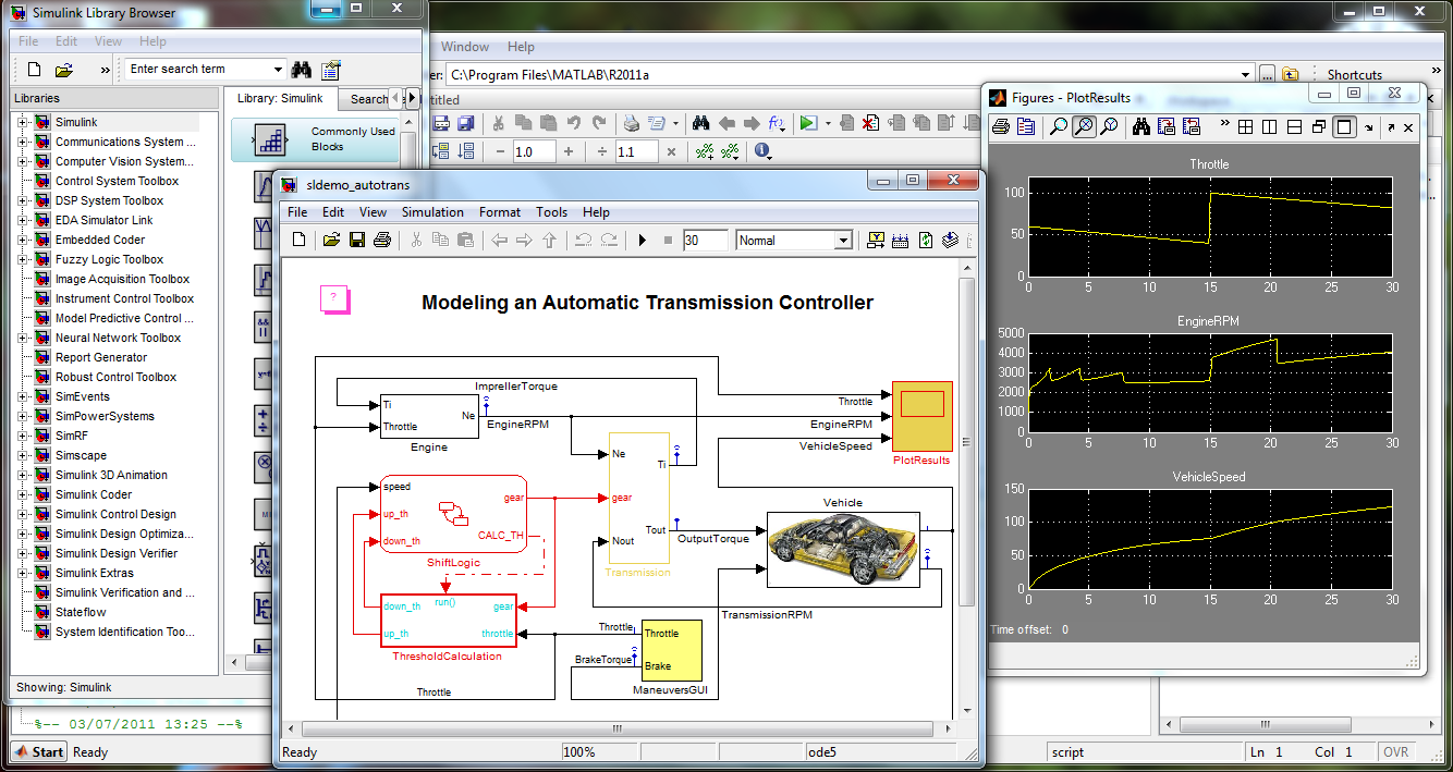
An example of the simulink interface

scala-flow is inspired by both of these tools. It is general purpose in the sense that it can be used to represent any dynamic systems. Nevertheless, its primary intended use is to develop, prototype, and debug embedded systems, and in particular those that make use of spatially programmed hardware. scala-flow has a functional/composable api, displays the constructed graph and provides block constructions. It has strong type safety: the type of the input and output of each node is checked during compilation time to ensure the soundness of the resulting graph.

Source, Sink and Transformations

Data are passed from nodes to nodes under the form of typed “packets” containing a value of the given type, an emission timestamp, and the delays the packet has encountered during its processing through the different nodes of the graph.

case class Timestamped[A](t: Time, v: A, dt: Time)

They are called Timestamped because they represent values and their corresponding timestamp information.

Packets get emitted from Source0[T] (nodes with no input), processed and transformed by other nodes until they reach sinks (nodes with no output). Nodes are connected between each other according to the structure of the data flow.

Nodes all mix-in the common trait Node. Every emitting Node (all nodes except sinks) mix-in the trait Source[A] whose type parameter A indicates the type of the packets emitted by this node. Indeed, nodes can only have one output but they can have any number of inputs. Every node also mixes-in the trait SourceX[A, B, ...] where X is the number of inputs for that node and is replaced by the actual arity (1, 2, 3, …). This is similar to FunctionX[A, B, ..., R], the type of functions in scala.

Source0 indicates that the node takes exactly 0 input.
Source1[A] indicates that the node has 1 input whose packets are of type A.
Source2[A,B] indicates that the nodes has 2 inputs whose packets are respectively of type A and B
etc …

Since all nodes mix-in a SourceX, the compiler can check that the inputs of each node are of the right type.

All SourceX must define def listenI(x: A) where I goes from 1 to X and A correspond to the corresponding type parameter of SourceX. def listenI(x: A) defines the action to take whenever a packet is received from the input I. Those functions are callbacks used to pass packets to the nodes following a listener pattern.

There is a special case, SourceN[A, R] which represent nodes that have an *-arity of type A and emit packets of type R. For instance, the Plot nodes take * number of sources and display them all on the same plot. The only constraint is that all the source nodes must emit the same kind of data of type A. Otherwise, it would not make sense to compare them. For plots specifically, A also has a context bound of Data which means that there exists a conversion from A to a Seq[Float], to ensure that A is displayable in a multiplot as time series. The x-axis, the time, correspond to the timestamp of emission contained in the packet.

An intermediary node that applies a transformation mixs-in the trait OpX[A, B, ..., R] where A, B is the type of the input, and R is the type of the output.

OpX[A, B, ..., R] extends SourceX[A, B, ...] with Source[R].

For instance, zip(sourceA, sourceB) is an Op[A, B, (A, B)]. In most cases, Ops are a transformation of an incoming packet followed by a broadcasting (with the function def broadcast(x: R)) to the nodes that have for source this node.

Demo

Below is the scala-flow code corresponding to a data-flow comparing a particle filter, an extended kalman filter, and the true state of the underlying model, the trajectory of the drone. At each tick of the different clocks, a packet containing the time as value is sent to a node simulating a sensor. Those sensors have access to the underlying model and transform the time into noisy sensor measurements, then forward them to the two filters. Once processed by the filters, the packets are plotted by the Plot sink. The plot also take as input the true state as given by the “toPoints” transformation.


  //****** Model ******
  val dtIMU   = 0.01
  val dtVicon = (dtIMU * 5)

  val covAcc    = 1.0 
  val covGyro   = 1.0 
  val covViconP = 0.1 
  val covViconQ = 0.1

  val numberParticles = 1200

  val clockIMU   = new TrajectoryClock(dtIMU)
  val clockVicon = new TrajectoryClock(dtVicon)

  val imu   = clockIMU.map(IMU(eye(3) * covAcc, eye(3) * covGyro, dtIMU))
  val vicon = clockVicon.map(Vicon(eye(3) * covViconP, eye(3) * covViconQ))

  lazy val pfilter = 
      ParticleFilterVicon(
        imu,
        vicon,
        numberParticles,
        covAcc,
        covGyro,
        covViconP,
        covViconQ
      )

  lazy val ekfilter = 
      EKFVicon(
        imu,
        vicon,
        covAcc,
        covGyro,
        covViconP,
        covViconQ
      )

  val filters = List(ekfilter, pfilter)

  val points = clockIMU.map(LambdaWithModel(
	(t: Time, traj: Trajectory) => traj.getPoint(t)), "toPoints")

  val pqs =  points.map(x => (x.p, x.q), "toPandQ")

  Plot(pqs, filters:_*)

Example of a scala-flow program

         ┌────────────────────┐ ┌────────────────────┐
         │TrajectoryClock 0.01│ │TrajectoryClock 0.05│
         └─────┬────────────┬─┘ └────────┬───────────┘
               │            │            │            
               v            v            v            
           ┌───────┐   ┌────────┐   ┌─────────┐       
           │Map IMU│   │toPoints│   │Map Vicon│       
           └──┬──┬─┘   └────┬───┘   └───┬──┬──┘       
              │  │          │           │  │          
              │  │          │    ┌──────┘  │          
              │  └──────────┼────┼─────────┼┐         
              └───────────┐ │    │         ││         
             ┌────────────┼─┘    │         ││         
             │            │      │         ││         
             v            v      v         vv         
         ┌───────┐ ┌───────────────────┐ ┌────────┐   
         │toPandQ│ │     RBPFVicon     │ │EKFVicon│   
         └───┬───┘ └──────────┬────────┘ └────┬───┘   
             │                │               │       
             └──────────────┐ │ ┌─────────────┘       
                            │ │ │                     
                            v v v                     
                          ┌───────┐                   
                          │ Plot  │                   
                          └───────┘

Graph representation of the data-flow

Block

A block is a node representing a group of nodes. That node can be summarized by its input and output such that from an external perspective, it can be considered as a simple node. Similar to the way an interface or an API hide its implementation details, a block hides its inner workings to the rest of the data-flow as long as the block receives and emits the right type of packets. This logic extends to the graphical representation. Blocks are represented as nodes in the high-level graph but expanded in an independent graph below the main one.

Similar to OpX[A, B, ..., R] , there exists BlockX[A, B, ..., R] which all extend Block[R] and take X sources as input. All Block[R] must define an out method of the form: def out: Source[R].

For instance, the filters are blocks with the following signatures:

case class RBPFVicon(rawSource1: Source[(Acceleration, Omega)],
                     rawSource2: Source[(Position, Attitude)],
                     N: Int,
                     covAcc: Real,
                     covGyro: Real,
                     covViconP: Real,
                     covViconQ: Real)	
	extends Block2[(Acceleration, Omega), 
		           (Position, Attitude),
				   (Position, Attitude)] {
	
		def imu = source1
		def vicon = source2
		
		def out = ...
	}

Signature of the block of the particle filter

and similar for EKFVicon.

The careful reader might notice that the above block takes as arguments rawSourceI and not sourceI directly. However, the packets are processing in the body of the class as incoming from sourceI (def imu = source1). This is a consequence of intermediary Source potentially needing to be generated during the graph creation to synchronize multiple scheduler together. More details below.

Graph construction

A graph can be entirely re-evaluated multiple times. For instance, we might want to run our simulation more than once. A feature of scala-flow is that the nodes of a graph are immutable and can be reused between different evaluations. This enables us to serialize, store or transfer a graph easily. A graph is a data structure and scala-flow follows that intuition by separating the construction of graph and its evaluations. What is specific and shortlived for the lapse of time of an evaluation of a graph are the Channels between the different nodes.

Channel

Channels are specific to a particular node and a particular “channel” of a node. A “channel” here refers to the actual I from listenI(packet) of a node to call. When the graph is initialized, the channels are created according to the graph structure.

If we take a look at Channel2 for instance:

sealed trait Channel[A] {
  def push(x: Timestamped[A], dt: Time): Unit
}

...

case class Channel2[A](receiver: Source2[_, A], scheduler: Scheduler)
    extends Channel[A] {
  def push(x: Timestamped[A], dt: Time = 0) = 
	...
}

We see that it requires that the receiver is a Source2. This actually means that the receiver must have at least (and not exactly) 2 sources. This is a consequence ofSourceI+1 extending SourceI, the base case being Source0: trait Source2[A, B] extends Source1[A].

Now, if we look at the private method broadcast inside Source[T]

  def broadcast(x: => Timestamped[A], t: Time = 0) =
    if (!closed)
      channels.foreach(_.push(x, t))

We see that broadcast is simply pushing elements into all its private channels. The channels are set during initialization of the graph in a simple manner: The graph is traversed and for all node the corresponding channel are created for its corresponding sources.

Buffer and cycles

It is possible to create cycles inside data-flows at the express condition that the immediate node creating a cycle is exclusively a kind of node called Buffer. Buffers relay to the next node any incoming data but with the particularity of a buffering of one packet. Buffers are created with an initial value. When the first packet arrives, the Buffer stores the incoming packet and broadcast the initial value. When another following packet arrives, the buffer stores the new packet and broadcast the previously stored one and so on.

Even using buffer nodes, declaring cycle requires additional steps:

val source: Source[A] = ...
val buffer = Buffer(merge, initA)
val zipped = source.zip(buffer)

This will not be valid scala because there is a circular dependency between buffer and zipped. Indeed, instantiating buffer require to instantiate zipped, which require to instantiate buffer … A solution is to use lazy val.

val source: Source[A] = ...
lazy val buffer = Buffer(merge, initA)
lazy val zipped = source.zip(buffer)

lazy val a = e in scala implements lazy evaluation, meaning the expression e is not evaluated until it is needed. In our case, this makes sure that both buffer and zipped can be declared and instantiated. It is enough that their parameters are declared of the right type, they do not actually need to evaluated. At the initialization of the entire graph, there is no circular dependency either because both instances exist and will only be used during the evaluation of the graph.

Source API

Here is a simplified description of the API of each source.

When relevant, the functions have an alternative methodNameT function that takes themselves function whose domain is Timestamped[A] instead of A.

For instance, there is a

def foreachT(f: Timestamped[A] => Unit): Source[A]

which is equivalent to the foreach below except it can access the additional fields t and dt in Timestamped


trait Source[A] {

  /** return a new source that map every incoming packet by the function f 
    * such that new packets are Timestamped[B] 
    */
  def map[B](f: A => B): Source[B]

  /** return a filtered source that only broadcast
    *  the elements that satisfy the predicate b */
  def filter(b: A => Boolean): Source[A]

  /** return this source and apply the function f to each
    *  incoming packets as soon as they are received 
    */
  def foreach(f: A => Unit): Source[A]
  
  /** return a new source that broadcast elements
    * until the first time the predicate b is not satisfied
    */
  def takeWhile(b: A => Boolean): Source[A]  
  
  /** return a new source that accumulate As into a List[A]
    * then broadcast it when the next packet from the other 
    * source clock is received 
    */
  def accumulate(clock: Source[Time]): Source[ListT[A]]
    
  /** return a new source that broadcast all element inside the collection
    * returned by the application of f to all incoming packet
    */
  def flatMap[C](f: A => List[C]): Source[C]
 
  /** assumes that A is a List[Timestamped[B]]. 
    * returns a new source that apply the reduce function 
    * over the collection contained in every incoming packet */
  def reduce[B](default: B, f: (B, B) => B)
      (implicit ev: A <:< ListT[B]): Source[B]
	  
  /** return a new source that broadcast pair of the packet from this source 
    * and the source provided as argument. Wait until a packet is received 
    * from both source. Packets from both source are queued such 
    * that independant of the order, they are never discarded
    * A2 B1 A3 B2 B3 B4 B5 A4=> (A1, B1), (A2, B2), (A3, B3), (A4, B4),
	* [Queue[B5]]
    */
  def zip[B](s2: Source[B]): Source[Boolean]


  /** return a new source that broadcast pair of the packet from this source 
    * and the source provided as argument. Similar to zip except that 
	* if multiple packets from the source provided as argument is received
	* before, all except the last get discarded.
    * A2 B1 A3 B2 B3 B4 B5 A4=> (A1, B1), (A2, B2), (A3, B3), (A4, B4),
	* [Queue[B5]]
    */
  def zipLastRight[B](s2: Source[B])

  
  /** return a new source that broadcast pair of the packet from this source 
    * and the source provided as argument. Similar to zip except that all 
	* packet except the last get discarded when both source are not in sync.
    * A1 A2 B1 A3 B2 B3 A4=> (A1, B1), (A3, B2), (B3, A4)
    */  
  def zipLast[B](s2: Source[B])

  /** return a new source that combine this source and the provided source .
    * packets from this source are Left
    * packets from the other source are Right
    */
  def merge[B](s2: Source[B]): Source[Either[A, B]]
  
  /** return a new source that fuse this source and the provided source
    * as long they have the same type.
    * any outgoing packet is indistinguishable of origin
    */  
  def fusion(sources: Source[A]*): Source[A]	  

  /** "label" every packet by the group returned by f */  
  def groupBy[B](f: A => B): Source[(B, A)]

  /** print every incoming packet */
  def debug(): Source[A]

  /** return a new source that buffer 1 element and 
    * broadcast the buffered element with the time of the incoming A 
    */
  def bufferWithTime(init: A): Source[A] 
  
  /** return a new source that do NOT broadcast any element */
  def muted: Source[A]

  /** return a new source that broadcast one incoming packet every 
    * n incoming packet.
    * The first broadcasted packet is the nth received one
    */
  def divider(n: Int): Source[A]

  /** return a pair of source from a source of pair */
  def unzip2[B, C](implicit ev: A <:< (B, C)): (Source[B], Source[C])
  
  /** return a new source whose every outgoing packet have an added dt
    * in their delay component
    */
  def latency(dt: Time): Source[A]

  /** return a new source whose broadcasted packets contain the time of 
    * emission
    */
  def toTime: Source[Time]

  /** return a new source that do NOT broadcast the first n packets */
  def drop(n: Int): Source[A]
}


implicit class TimeSource(source: Source[Time]) {

  /** stop the broadcasting after the timeframe tf has elapsed */
  def stop(tf: Timeframe): Source[Time]

  /** add a random delay following a gaussian with corresponding 
    * mean and variance */
  def latencyVariance(mean: Real, variance: Real): Source[Time]

  /** add a delay of dt */
  def latency(dt: Time): Source[Time]

  /** return a new source of the difference of time between 
    * the two last emitted packets */
  def deltaTime(init: Time = 0.0): Source[Time]
  
}

API of the Sources

The real API also includes name and silent parameters. Both are only relevant for the graphical representation. The name of the block will be overriden by name if present and the node will be skipped in the graphical representation if silent is present.

Batteries

The following nodes are already included and pre-defined:

Clock: Source0[Time] that takes as parameter a timeframe dt which corresponds to the lapse of time between each emission of packets. The packets contain as values the time of emission.
TestTS: “Test Time Series” Sink that takes a source of labeled data. Labeled data are data joined with their corresponding label. This sink displays the mean error, the max error error across all datapoints and also the RMSE.
```
[info ParticleFi ] RMSE       : 1.099241e-01, 4.213478e-03
[info ParticleFi ] Mean errors: 3.026816e-01, 4.746430e-02
[info ParticleFi ] Max  errors: 7.086643e-01, 2.386466e-01
```
Plot: Sink that displays the time series under the form of a plot. Can take an arbitrary number of time series, each of arbitrary dimension. In the example below, 5 time series of 2 dimensions are plotted. The plotting library is the one included in scala-breeze, used elsewhere for matrix and vector operations.

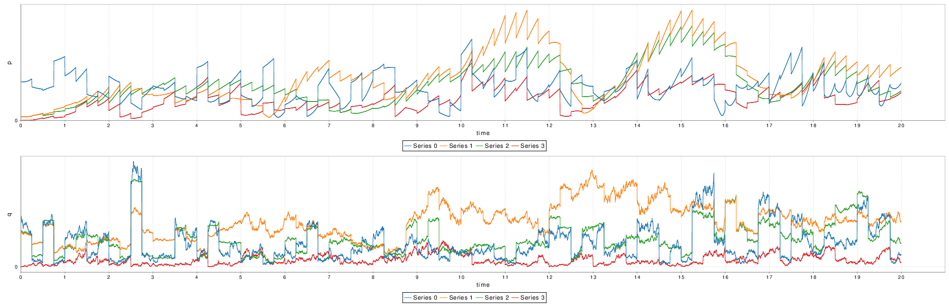
Example of a plot generated by the Plot sink

Jzy3dTrajectoryVisualisation: Sink. It displays a point following a trajectory in a new window. takes a source of points as source. An example as shown in Part I.

Example of a trajectory visualization

In addition, any scala.Stream[A] can be transformed into a Source0 node using EmitterStream[A] with A being the type of the Stream. This is how Clock is implemented, as an infinite scala stream of Time.

Batch

A batch is a node that processes its inputs in “batch” mode. All the other nodes process their inputs in “stream” mode. By “stream” mode, it is meant that the node processes the inputs one-by-one, as soon as they arrive. On the other hand, the “batch” mode means that the node processes the incoming packets once they have all arrived, once and for all. This is the case for most sinks (for example, it makes more sense for a plot to build it once all the data is arrived).

Spatial is a language described in part IV and developed to write high-level hardware design of accelerators. A spatial application can be integrated into scala-flow as a transformation node using the streaming interface of Spatial. Spatial applications can only run during the same runtime than scala-flow using the interpreter described in Part III and originally developed for this exact purpose. Batches are essential to Spatial integration: the nodes that simulate a Spatial application can only run and treat all the data at once. Indeed, running a Spatial application involves running the Spatial compiler in the background and compiling the full meta-program, including all meta-constant values.

Scheduler

Scheduling is the core mechanism of scala-flow. Scheduling ensures that packets get emitted by the sending nodes and received by the recipient nodes at the “right time”. Since scala-flow is a simulation tool, the “scala-flow time” does not correspond at all to the real time. Scheduling emits the packets as fast as it can. Therefore, since time is an arbitrary component of the packet, the only constraint that scheduling must satisfy is emitting the packets from all nodes in the right order.

Scheduling is achieved by one or many Schedulers. Schedulers are essentially priority queues of actions. The priority is the timestamp plus the accumulated delay of the packet. The actions are side-effect functions that emit packets to the right node by the intermediary of channels. Every node has a scheduler and enqueue action to it every time the broadcast method is called. The scheduler are propagated through the graph through two rules:

Every Source0 has for Scheduler the “main scheduler” available globally passed on as an implicit parameter
Other nodes either explicitly create their own scheduler (like the batch nodes) or use the Scheduler from their source1 input.

Only one scheduler executes actions at the same time. When a scheduler is finished, another one is started unless it was the last one. In practice, when a scheduler has no more packets to handle, there is a callback to CloseListener nodes and scheduler according to their CloseListener priority. Batches have their own scheduler and are also among CloseListener of the Scheduler of their source node, waiting for them to all finish. Batches process the accumulated packets as soon as the CloseListener callback is called.

All schedulers start at time 0. The current time of a scheduler is the time of the last emitted packet. Scheduler can en-queue new actions while the scheduler is “live” but the en-queued packet can only have a time of emission greater or equal to the current time. In the trivial case where there is no Batch, only one scheduler is needed.

Replay

Replay are nodes at the frontier of two schedulers. They accumulate packets from the actions of the first scheduler until they receive its CloseListener callback. When received, they en-queue all the accumulated actions into the second scheduler. Replays are the primary mechanisms of synchronization between two Schedulers. A Batch is essentially a Replay with its own Scheduler as secondary Scheduler. However, a batch transforms the data before broadcasting instead of simply replaying it.

All sources of a node must share the same scheduler. Replays are automatically inserted to ensure that this rule is respected

The automatic insertion is the reason why nodes must define all rawSourceI but one should only externally ever use the sourceI methods. In most case, rawSourceI and sourceI are by definition the same. However, if a replay node has to be created, it is inserted in-between rawSourceI and sourceI.

Multi-Scheduler graph

When the graph involves multiple schedulers, depending on the graph structure, the synchronization between them might require additional replays.

graph LR subgraph scheduler 1 sA(sourceA) sB(sourceB) sC(sourceC) end subgraph scheduler2 node(Node) rest(...) end sA-->node sB-->node sC-->node node-->rest

Node’s sources sharing the same Scheduler

In the above structure, no replay need to be created because all sources of the node “Node” share the same scheduler. It suffices to wait for the closing callback of that scheduler.

graph LR subgraph scheduler 1 sA(sourceA) end subgraph scheduler 2 sB(sourceB) end subgraph scheduler 3 sC(sourceC) end subgraph scheduler 4 node(Node) rest(...) end sA-->node sB-->node sC-->node node-->rest

Node’s sources not sharing the same Scheduler

In the above structure, intermediary replays must be created so that the node “Node” sources share the same scheduler.

graph LR subgraph scheduler 1 sA(sourceA) end subgraph scheduler 2 sB(sourceB) end subgraph scheduler 3 sC(sourceC) end subgraph scheduler 4 replay1(Replay1) replay2(Replay2) replay3(Replay3) end subgraph scheduler 5 node(Node) rest(...) end sA-->replay1 sB-->replay2 sC-->replay3 replay1-->node replay2-->node replay3-->node node-->rest

Example of Replays between inserted in-between a Node and its sources

InitHook

Some nodes need initialization values for each simulation evaluation. For instance, this is the case for the trajectory filters: the filters require to be given the initial position and attitude of the drone. An InitHook[I] is an implicit parameter passed to the nodes during their declaration. The type parameter I is the type of the values that will be accessible by the nodes as initialization values.

ModelHook

Similarly, some nodes need access to a “Model”. A “Model” is specific to a simulation and is an oracle that a node might need to consult in order to generate data or get any other information about the external simulation environment. For instance, the sensor nodes generate noisy measurements as a function of the time based on the underlying trajectory model. Similar to InitHook[I], it is passed to nodes during the graph declaration as an implicit parameter.

NodeHook

To gather the nodes and their connection between each others, a NodeHook is used. Every node must have access to a NodeHook to add itself to the registry. For nodes that take no input, the Source0, the NodeHook is passed as an implicit parameter. For any other nodes, the NodeHook is propagated through the graph. All others nodes use the NodeHook from their source1. This is similar to the way Scheduler are propagated through the graph.

Graphical representation

The graphical representation is a graph in the ASCII format. The library ascii-graphs is used to generate the output in ASCII from sets of vertices and edges. The set of vertices and edges is retrieved from the set of nodes contained in NodeHook and their sources.

FlowApp

A FlowApp[M, I] is an extension of the scala App, a trait that treats the inner declaration of an object as a main program function. Its type parameters correspond respectively to the type parameter of ModelHook[M] and InitHook[I]. A FlowApp has the methods drawExpandedGraph() which display the ASCII representation of the graph and the method run(model, init) which run the evaluation of the simulation with the given model and initialization value.

Spatial integration

Scala-flow can also be used as a complementary tool for the development of applications embedding Spatial, a language to design hardware accelerators. Accelerators can be easily represented as simple transformation nodes in a data flow and hence as a regular OpX node in scala-flow.

SpatialBatch and its variants are the nodes used to embed spatial applications. SpatialBatchRawXs run a user-defined application. The application can use the list of incoming packets as a constant list of values. X is the number of sources of the node. SpatialBatchXs are specialized SpatialBatchRawXs with additional syntactic sugar such that there is no more boilerplate and the required code is reduced to the most essential to write stream processing Spatial applications. It is only to define a function def spatial(x: TSA): SR where TSA is a struct containing a value v of type SA (see below) and the packet timestamp as t.

If we take a look at SpatialBatch1’s signature,

abstract class SpatialBatch1[A, R, SA: Bits: Type, SR: Bits: Type]
	(val rawSource1: Source[A])
	(implicit val sa: Spatialable[A] { type Spatial = SA },
			  val sr: Spatialable[R] { type Spatial = SR }
	)

we see that it takes type parameter A, R, SA, SR and the typeclass instances of Spatialable for SA and SR. A and R are the type members representing respectively the incoming and outgoing packet type. SA and SR are the spatial type into what they are converted to such that they can be handled by a spatial DSL. Indeed, scala.Double and spatial.Double are not the same type. The latter is a staged type part of the spatial DSL.

Spatialable[A] is a typeclass that declare a conversion from A to a Spatial type (declared as the inner type member Spatial of Spatialable.

There exists a Spatialable[Time] which make the following example possible:

  val clock1 = new Clock(0.1).stop(10)
  val clock2 = new Clock(0.1).stop(10)  

  val spatial = new SpatialBatch1[Time, Time, Double, Double](clock1) {
    def spatial(x: TSA) = {
      cos(x.v)
    }    
  }

  val spatial2 = new SpatialBatch1[Time, Time, Double, Double](clock2) {
    def spatial(x: TSA) = {
      x.v + 42
    }    
  }


  val spatial3 = new SpatialBatch2[Time, Time, Time, Double, Double, Double]
	                              (spatial, spatial2) {
    def spatial(x: Either[TSA, TSB]) = {
      x match {
        case Right(t) => t.v+10
        case Left(t) => t.v-10
      }
    }    
  }

  Plot(spatial3)

Usage demonstration of spatial batches

Even though it looks inconspicuous, the cos, +, - functions are actually functions from the Spatial DSL. This simple scala-flow program actually compiles and runs through the interpreter 3 different Spatial programs.

The development of an interpreter was required so that Spatial applications could run on the same runtime than scala-flow. The interpreter development is detailed in the next part of this thesis.

Conclusion

scala-flow is a modern framework to simulate, develop, prototype and debug applications which have a natural representation as data-flows. Its integration with Spatial makes it a good tool to include with Spatial to ease the development complex applications whenever the accelerated application needs to be written over multiple iterations of increasing complexity, and tested on different scenarios with modelable environments.

Part III

Continue here to read the section about an interpreter for Spatial (III/IV)