(thesis 4/4) The Spatial implementation of a Rao-Blackwellized Particle Filter

Posted on August 16, 2017 by Ruben Fiszel

About

This post is the part IV out of IV of my master thesis at the DAWN lab, Stanford, under Prof. Kunle and Prof. Odersky supervision. The central themes of this thesis are sensor fusion and spatial, an hardware description language (Verilog is also one, but tedious).

This part is about the spatial implementation of the asynchronous Rao-Blackwellized Particle filter presented in part I.

Spatial implementation of an asynchronous Rao-Blackwellized Particle Filter

A Rao-Blackwellized Particle Filter turned out to be an ambitious application, the most complex that was developed so far with Spatial. It is an embarrassingly parallel algorithm and hence can leverage the parallelizable benefits of an application-specific hardware design. Developing this, we gained some insights specific about the hardware implementation of such an application and some others specific to the particularities of Spatial. At the time of the writing, some Spatial incomplete codegen prevented full synthesis of the application, but it ran correctly in the simulation mode and the area usage estimation fit on a Zynq board.

Area

The capacity of an FPGA is defined by its total resources: the synthesizable area and the memories. Synthesizable area is defined by the number of logic cells. Logic cells simulate any of the primitive logic gates through a lookup table (LUT).

Memories are Scratchpad memory (SPM), high-speed internal writable cells used for temporary storage of calculations, data, and other work in progress. SPM are divided into 3 kinds:

BRAM is a single cycle addressable memory that can contain up to 20Kb. There are commonly on the order of magnitude of up to a thousand BRAM.
DRAM is burst-addressable (up to 512 bits at once) off-chip memory that has a capacity on the order of Gb. The DRAM is visible to the CPU and can be used as an interface mechanism to the FPGA.
Registers are single elements memory (non-addressable). When used as part of a group of registers, they make possible parallel access.

Parallel patterns

Parallel patterns [1] are a core set of operations that capture the essence of possible parallel operations. The 3 most important one are:

FlatMap
Fold

filter is also an important pattern but can be expressed in term of a flatMap (l.flatMap(x => if (b(x)) List(x) else Nil)). Foreach is a Fold with a Unit accumulator. Reduce can be expressed as a Fold (The Reduce operator from Spatial is actually a fold that ignores the accumulator on the first iterator). By reducing these patterns to their essence, and offering parallel implementations for them, Spatial can offer powerful parallelization that fits most, if not all, use-cases.

In Spatial, FlatMap is actually composed by chaining a native Map and a FIFO.

Control flows

Control flows (or flow of control) is the order in which individual statements, instructions or function calls of an imperative program are executed or evaluated. Spatial offers 3 kinds of Control flows.

Spatial has hierarchical loop nesting. When loops are nested, every loop is an outer loop except the innermost loop. When there is no nesting, the loop is an inner loop. Control flows are outer loop annotations in Spatial. The 3 kind of annotation are:

Sequential: The set of operations inside the annotated outer loop is done in sequence, one after the other. The first operation of the next iteration is never started before the last operation of the current iteration. syntax: parallel pattern annotation Sequential.Foreach ...
Parallel: The set of operations inside the annotated body is done in parallel. Loops can be given a parallelization factor, which creates as many hardware duplicates as the parallelization factor.
syntax: Parallel { body }, parallel counter annotation (0 to N par parFactor).
Pipe: The set of inner operations is pipelined Divided in 3 subkinds:
- Inner Pipe: Basic form of pipelining; Only chosen when all the inner operations are primitive operations and hence, no buffering is needed.
- Coarse-Grain: Pipelining of parallel patterns: When loops are nested, a coarse-grain retiming and buffering must be done to increase the pipe throughput syntax: Pipe { body } or for parallel pattern annotation Pipe.Foreach ....
  Syntax is shared for Inner pipe or Coarse-grain but chosen depending on whether the inner operations are all “primitives” or not
- Stream Pipe: As soon as an operation is done, it must be stored in an hardware unit that support a FIFO interface (enqueue, dequeue), such that the pipelining is always achieved in an as soon as possible manner. Use the Stream syntax syntax: Stream { body } or for parallel pattern annotation Stream.Foreach ...

When not annotated, the outer loop is a Pipe by default.

${lang-ref}

Numeric types

Numbers can be represented in two ways:

fixed-point: In the fixed-point representation, an arbitrary number of bits I represent the integer value, an arbitrary number of bits D represent the decimal value. If the representation is signed, negative numbers are represented using 2’s complement.

I defines the range (the maximum number that can be represented) and D defines the precision. The range is centered on 0 if the representation is signed.

In Spatial, the fixed-point type is declared by FixPt[S: _BOOL, I: _INT, D: _INT].
_BOOL is the typeclass of the types that represents a boolean. true and false types are _TRUE and _FALSE.
Likewise for_INT,the typeclass of types that represent a literal integer. The integers from 0 to 64 have the corresponding types _0, _1, …, _64.

floating-point: In the floating-point representation, one bit represents the sign, an arbitrary number of bits E represent the exponent and an arbitrary number of bits represent the significand part.

In Spatial, the floating-point type is declared by FltPt[S: _INT, E: _INT].

By comparison, in the software world, the commonly available numeric types for integers are fixed points: Byte (8-bits), Short (16-bits), Int (32-bits), Long (64-bits) and for real floating-point: Float (32-bits), Double (64-bits).

The floating-point representation is required for some applications because its precision increases as we get closer to 0: the space between all representable numbers around 0 diminish whereas it is uniform over the whole domain for the fixed point representation. This can be extremely important to store probabilities (since joint probability, when not normalized, can be infinitesimally small), or to store the result of exponentiation of negative numbers (a small difference in value might represent a big difference pre-exponentiation), or to store the values of square (we need more precision the closest we are from 0 because the line of the real squared is more “dense” the closer we are from 0). However, floating-point operations utilize more area resources than fixed-point (an increase by an order of magnitude of around 2)

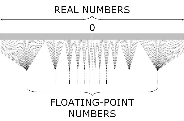
Representable Real line and its corresponding floating-point representation

Fortunately, in Spatial, it is easy to define a type Alias to gather all the values that should share the same representation and then switch from floating-point to the fixed-point representation and tune the allocated number of bits by editing solely the type alias.

//only this line need to be edited to change the representation
type SmallReal = FixPt[_TRUE, _4, _16]

val a: SmallReal = ...
val b: SmallReal = ...

Vector and matrix module

The state and uncertainty of a particle are a vector and a matrix (the matrix of covariance). All the operations involving the state and uncertainty, in particular Kalman prediction and Kalman update are matrix and vector operations. Kalman updates, for instance, when written in the matrix form is reasonably compact in the matrix form but actually represents a significant amount of compute and operations. For the sake of code clarity, it is crucial to be able to keep being able to write matrix operations in a succinct syntax. Furthermore, matrix and vector operations are a common need and it would be beneficial to write a reusable set of operations to Spatial. This is why a vector and matrix module was developed and added to the standard library of Spatial. The standard library is inaugurated by this module and its purpose is to include all the common set of operations that should not be part of the API because they do not constitute primitives of the language. Modules of the stdlib (standard library) are individually imported based on the needs.

Matrix operations currently available are +, -, * (element wise when applied to a scalar, else matrix multiplication), .transpose .det (matrix determinant), .inverse, h (matrix height), w (matrix width). Vec operations currently available are +, -, * (element-wise with a scalar), .dot (dot-product).

In place operations exists for +, -, * as :+, :-, :*. In place operations use the RegFile of the first element for the output instead of creating a new RegFile. This should be used with care because it makes pipelining much more inefficient (since the register is written twice to with a long delay in-between corresponding the operation).

Matrix and Vec operations are parallelized whenever loops are involved.

Meta-Programming

Matrices and Vectors are stored as RegFile[Real] with the corresponding dimension of the matrix. However, from a user perspective, it is preferable to manipulate a type that corresponds to the abstraction, here a vector or matrix. We can achieve this with a wrapper type with a no-cost abstraction thanks to meta-expansion. Those wrapper types are hybrid types mixing staged (for the dimension) and non-staged types (for the data). Indeed, the staging compiler only sees the operations on the RegFile directly.

Here is a simplified example.

case class Vec(size: scala.Int, data: RegFile[Real]) {
	def +(y: Vec) = {
		require(y.size == size)
		val nreg = RegFile[T](n)
		Foreach(0::n){ i =>
			nreg(i) = data(i) + y.data(i)
		}
      copy(data = nreg)
	}
		
		
}

val v = Vec.fill(3)
v + v

We can observe the require(y.size == size). Since size is a non-staged type, the dimension is actually checked during meta-expansion. Similarly, matrix sizes are checked for all operations and the dimensions are propagated to the resulting matrix (e.g: Mat(a, b)*Mat(b,c) = Mat(a,c)). It prevents early a lot of issues.

Furthermore, the Matrix API containing common matrix operations is implemented by 3 classes:

MatrixDense for matrices with dense data
MatrixSparse for matrices with sparse data. Optimizes operations by not doing unnecessary additions and multiplications when empty cells are involved.
MatrixDiag for diagonal matrices. Provide constant operations for multiplications with other matrices by only modifying a factor component. Use only 1 register for the whole matrix as a factor value.

The underlying implementation are hidden from the user since they are all created from the Matrix companion object. Then, the most optimized type possible is conserved through the transformation. When impossible to know the structure of the new matrix, the fallback is MatrixDense.

Views

Some operations like transpose and many others do not need to actually change the matrix upon which they are realized. They could just operate on a view of the underlying RegFile memory. This view is also a no-cost abstraction since it does not exist after meta-expansion.

Here is a simplified example.

sealed trait RegView2 {
  def apply(y: Index, x: Index)(implicit sc: SourceContext): T
  def update(y: Index, x: Index, v: T)(implicit sc: SourceContext): Unit      
}  

case class RegId2(reg: RegFile2[T]) extends RegView2 {
  def apply(y: Index, x: Index)(implicit sc: SourceContext) =
    reg(y, x)
  def update(y: Index, x: Index, v: T)(implicit sc: SourceContext) =
    reg(y, x) = v      

}  

case class RegTranspose2(reg: RegView2) extends RegView2 {
  def apply(y: Index, x: Index)(implicit sc: SourceContext) = reg(x, y)
  def update(y: Index, x: Index, v: T)(implicit sc: SourceContext) =
    reg(x, y) = v
  
}

case class MatrixDense(h: scala.Int, w: scala.Int, reg: RegView2) extends Matrix {

  def toMatrixDense = this

  def apply(y: Index, x: Index)(implicit sc: SourceContext) = {
    reg(y, x)
  }

  //The transpose operation do not actually do any staged operations.
  //It simply invert the y and x dimension for update and access.
  def t =
    copy(h = w, w = h, reg = RegTranspose2(reg))
}

In the same spirit, views exist for SRAM access, constant values, vec as diagonal matrix, matrix column as vec, matrix row as vec.

Mini Particle Filter

A “mini” particle Filter has been developed at first. The model has been simplified. It supposes that the drone always has the same normal orientation and only moves in 2D, on the x and y axis. The state to estimate is only the 2D position. It is a plain particle filter and therefore, not conditioned on a latent variable and without any Kalman filtering. Thus, no matrix operations need to be applied. The sensor measurements are stored and loaded directly as constant values in the DRAM. This filter is a sanity check that the particle filter structure is sound, fittable on a Zynq board and working as expected.

The full Mini Particle Filter source code application is contained in the Appendix and publicly available as a Spatial application on github.

Rao-Blackwellized Particle Filter

The RBPF implementation on hardware follows the expected structure of the filter thanks to Spatial’s high level of abstraction. To implement the sensors needing to be processed in order, one FIFO is assigned for each sensor. Then an FSM dequeues and updates the filter one measurement at a time. The dequeued FIFO is the one containing the measurement with the oldest timestamp. This ensures that measurements are always processed one at a time and in order of creation’s timestamp.

The full Rao-Blackwellized source code application is contained in the Appendix and publicly available as a Spatial application on github.

Insights

When writing complex applications, one must be careful about writing functions. Indeed, functions are always applied and inlined during meta-expansion. This results in the IR growing exponentially and causes the compiler phase to take a long time. Staged functions will be brought to Spatial to reduce the IR exponential growth in the future. However, the intrinsic nature of hardware must result in function application being “inlined” since the circuit are by definition duplicated when synthesized. This is why, factoring should not be done the same way in Spatial as in Software. In Software, a good factorization rule is to avoid all repetition of the code by generalizing all common parts into functions. For Spatial, the factorization must be thought of as avoiding all repetition of the synthesized hardware by reusing as many memories, signal and wires as possible.
Changing the numeric type matters: floating-point operations are much costlier in term of area than fixed-point and should be used with parsimony when the area resources are limited.
Parallelization can be achieved through pipelining. Indeed, a pipeline will attempt to use all the resources available in parallel. Compared to duplicating hardware, a pipeline only takes at most N the biggest time steps of the pipeline. If the time step is small enough compared to the entire time length of the pipeline, the time overhead is small and no area is wasted.
Doing in-place operations seems like a great idea to save memory at first, but it breaks pipelining so it has to be used with caution.
Reducing the number of operations between first and last access is crucial because the number of operation correspond to the depth of the pipeline. When the depth grows large, coarse grain pipelining will have to create as many intermediate buffers to ensure protected access at different stages of the pipeline. Furthermore, the order of execution is currently not rearranged by the compiler, so, in some cases, simply changing the order of a few line of codes can make a tremendous difference in the depth of the pipeline.

Conclusion

The Rao-Blackwellized Particle Filter is a complex application. It would have been impractical, almost to the point of infeasible, to attempt to build it with a reasonable latency and throughput, in a timely manner, for a single person, if not for Spatial. We also gained insights about the development of complex applications for spatial and developed a new Matrix module as part of the standard library that might ease the development of new Spatial applications.

Conclusion

This work presents a novel approach to POSE estimation of drones with an accelerated, asynchronous, Rao-Blackwellized Particle Filter and its implementation in software and hardware. A Rao-Blackwellized Particle Filter is mathematically more sound to solve the complexities of tracking the non-linear transformations of the orientation through time than current alternatives. Furthermore, we show that this choice improves upon the accuracy for both the position and orientation estimation.

To exploit the inherent parallelism in the filter, we have developed a highly accurate hardware implementation in Spatial with low latency and high throughput, capable of handling highly dynamic settings such as drone tracking.

We have also developed two components that ease the design of hardware data paths for streaming applications; Scala-flow, a standalone data-flow simulation tool, and an interpreter for Spatial that can execute at staging time any arbitrary Spatial program. The interpreter is a key component to enable integration of the hardware programmability of Spatial to the streaming capabilities of Scala-flow. Scala-flow offers a functional interface, accurate functional simulation, hierarchical and modular grouping of nodes through blocks, immutable representation of the data flow graph, automatic batch scheduling, a graph structure display, interactive debugging and the ability to generate plots.

On a higher level, this work shows that Scala, being the underlying language substrate behind Spatial, enables building complex and extensive development tools without sacrificing productivity. It also shows that Spatial is a powerful, productive, and versatile language that can be used in a wide range of applications, such as extending the current state-of-the-art of embedded drone applications.

References

[1] R. Prabhakar, “Generating configurable hardware from parallel patterns,” ACM SIGOPS Operating Systems Review, vol. 50, no. 2, pp. 651–665, 2016.