About

This post is the part I out of IV of my master thesis at the DAWN lab, Stanford, under Prof. Kunle and Prof. Odersky supervision. The central themes of this thesis are sensor fusion and spatial, an hardware description language (Verilog is also one, but tedious).

This part is about an application of hardware acceleration, sensor fusion for drones. Part II will be about scala-flow, a library made during my thesis as a development tool for Spatial inspired by Simulink. This library eased the development of the filter but is also intended to be general purpose. Part III is about the development of an interpreter for spatial. Finally, Part IV is about the spatial implementation of the asynchronous Rao-Blackwellized Particle filter presented in Part I. If you are only interested in the filter, you can skip the introduction.

Introduction

The decline of Moore’s law

Moore’s law¹ has prevailed in the computation world for the last four decades. Each new generation of processor comes the promise of exponentially faster execution. However, transistors are reaching the scale of 10nm, only one hundred times bigger than an atom. Unfortunately, the quantum rules of physics governing the infinitesimally small start to manifest themselves. In particular, quantum tunneling moves electrons across classically insurmountable barriers, making computations approximate, resulting in a non negligible fraction of errors.

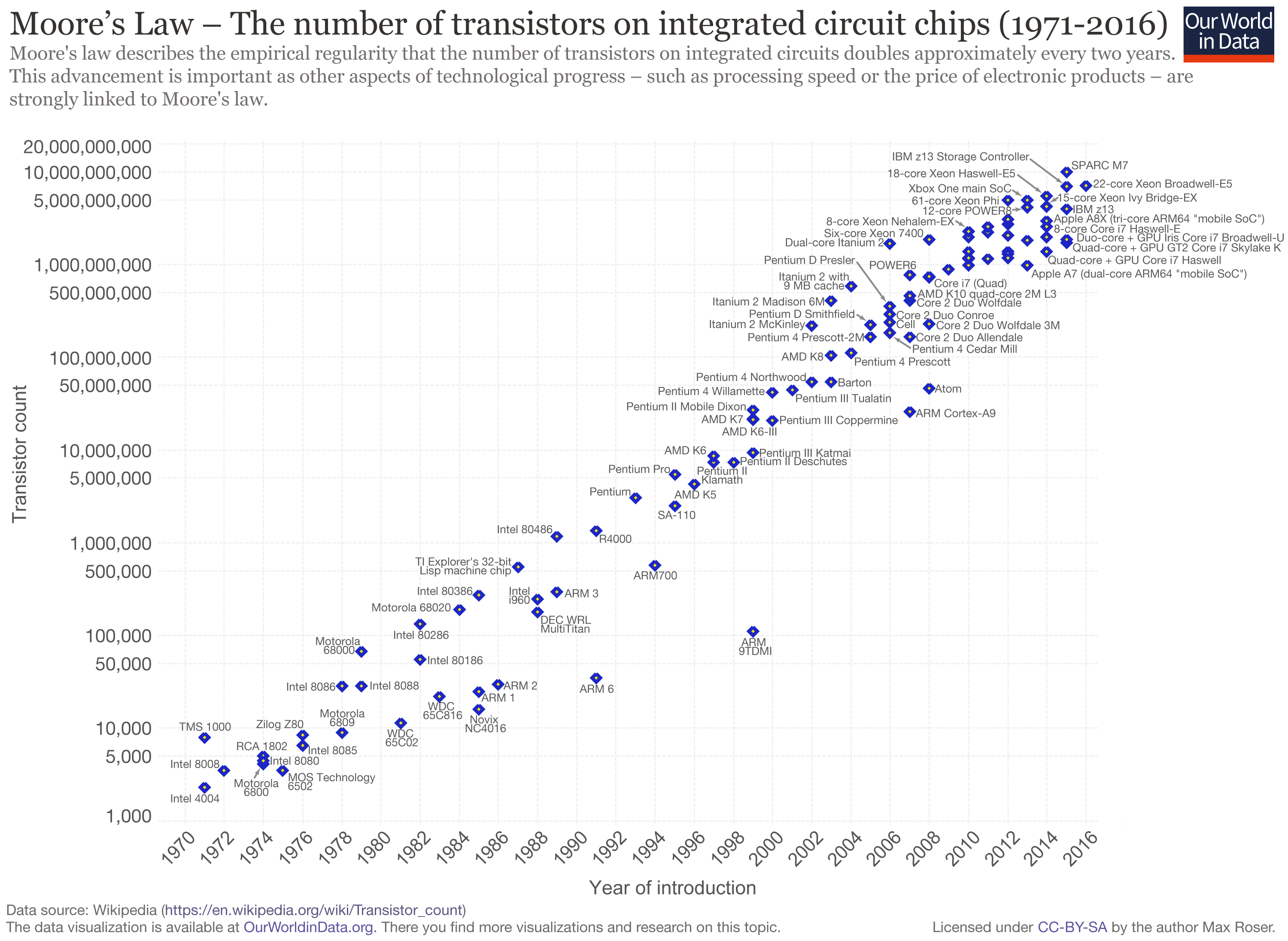
The number of transistors throughout the years. We can observe a recent start of a decline

The rise of Hardware

Hardware and Software respectively describe here programs that are executed as code for a general purpose processing unit and programs that are a hardware description and synthesized as circuits. The dichotomy is not very well-defined and we can think of it as a spectrum. General-purpose computing on graphics processing units (GPGPU) is in-between in the sense that it is general purpose but relevant only for embarrassingly parallel tasks² and very efficient when used well. GPUs have benefited from high-investment and many generations of iterations and hence, for some tasks they can match with or even surpass hardware such as field-programmable gate arrays (FPGA).

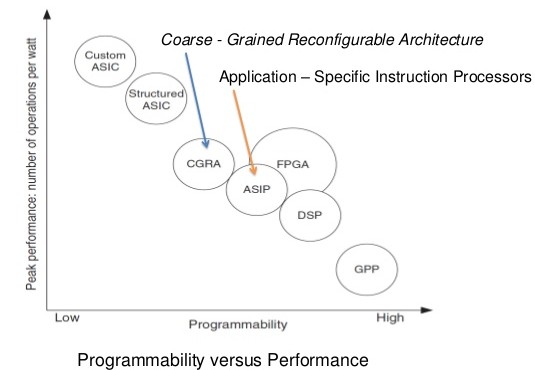
Hardware vs Software

The option of custom hardware implementations has always been there, but application-specific integrated circuit (ASIC) has prohibitive costs upfront (near $100M for a tapeout). Reprogrammable hardware like FPGAs have only been used marginally and for some specific industries like high-frequency trading. But now Hardware is the next natural step to increase performance, at least until a computing revolution happens, e.g: quantum computing, yet this sounds unrealistic in a near future. Nevertheless, hardware do not enjoy the same quality of tooling, language and integrated development environments (IDE) as software. This is one the motivations behind Spatial: bridging the gap between software and hardware by abstracting control flow through language constructions.

Hardware as companion accelerators

In most cases, hardware would be inappropriate: running an OS as hardware would be impracticable. Nevertheless, as a companion to a central-processing unit (CPU also called “the host”), it is possible to get the best of both worlds: the flexibility of software on a CPU with the speed of hardware. In this setup, hardware is considered an “accelerator” (hence, the term “hardware accelerator”). It accelerates the most demanding subroutines of the CPU. This companionship is already present in modern computer desktops in the form of GPUs for shader operations and sound cards for complex sound transformation/output.

The right metric: Perf/Watt

The right evaluation metric for accelerators is performance per energy, as measured in FLOPS per Watt. This is a fair metric for comparing different hardware and architecture because it reveals its intrinsic properties as a computing element. If the metric was solely performance, then it would be enough to stack the same hardware and eventually reach the scale of a super-computer. Performance per dollar is not a good metric either because it does not account for the cost of energy at runtime. Hence, Perf/Watt is a fair metric to compare architectures.

Spatial

At the DAWN lab, under the lead of Prof. Olukotun and his grad students, is developed an Hardware Description Language (HDL) implemented as an embedded scala DSL spatial and its compiler to program Hardware in a higher-level, more user-friendly, more productive language than Verilog. In particular, control flows are automatically generated when possible. This should enable software engineers to unlock the potential of Hardware. A custom CGRA, Plasticine, has been developed in parallel to Spatial. It leverages some recurrent patterns as the parallel patterns and it aims at being the most efficient reprogrammable architecture for Spatial.

Th upfront cost is large but once at a big enough scale, Plasticine could be deployed as an accelerator in a wide range of use-cases, from the most demanding server applications to embedded systems with heavy computing requirements.

Embedded systems and drones

Embedded systems are limited by the amount of power at disposal in the battery and may also have size constraints. At the same time, especially for autonomous vehicles, there is a great need for computing power.

Thus, developing drone applications with Spatial demonstrates the advantages of the platform. As a matter of fact, the filter implementation was only made possible because it is run on a hardware accelerator. It would be unfeasible to run it on more conventional micro-transistors. Particle filters, the family of filter which encompasses the types developed here, being very computationally expensive, are very seldom used for drones.

Sensor fusion algorithm for POSE estimation of drones: Asynchronous Rao-Blackwellized Particle filter

POSE is the combination of the position and orientation of an object. POSE estimation is important for drones. It is a subroutine of SLAM (Simultaneous localization and mapping) and it is a central part of motion planning and motion control. More accurate and more reliable POSE estimation results in more agile, more reactive and safer drones. Drones are an intellectually stimulating topic and in the near-future they might also see their usage increase exponentially. In this context, developing and implementing new filter for POSE estimation is both important for the field of robotics but also to demonstrate the importance of hardware acceleration. Indeed, the best and last filter presented here is only made possible because it can be hardware accelerated with Spatial. Furthermore, particle filters are embarrassingly parallel algorithms. Hence, they can leverage the potential of a dedicated hardware design. The Spatial implementation will be presented in Part IV.

Before expanding on the Rao-Blackwellized Particle Filter (RBPF), we will introduce here several other filters for POSE estimation for highly dynamic objects: Complementary filter, Kalman Filter, Extended Kalman Filter, Particle Filter and finally Rao-Blackwellized Particle filter. This ranges from the most conceptually simple, to the most complex. This order is justified because complex filters aim to alleviate some of the flaws of their simpler counterparts. It is important to understand which one and how.

The core of the problem we are trying to solve is to track the current position of the drone given the noisy measurements of the sensor. It is a challenging problem because a good algorithm must take into account that the measurements are noisy and that the transformation applied to the state are non-linear, because of the orientation components of the state. Particle filters are efficient to handle non-linear state transformations and that is the intuition behind the development of the RBPF.

All the following filters are developed and tested in scala-flow. scala-flow will be expanded in part II of this thesis. For now, we will focus on the model and the results, and leave the implementation details for later.

Drones and collision avoidance

The original motivation for the development of accelerated POSE estimation is for the task of collision avoidance by quadcopters. In particular, a collision avoidance algorithm developed at the ASL lab and demonstrated here (https://youtu.be/kdlhfMiWVV0)

Ross Allen fencing with his drone

where the drone avoids the sword attack from its creator. At first, it was thought of accelerating the whole algorithm but it was found that one of the most demanding subroutines was pose estimation. Moreover, it was wished to increase the processing rate of the filter such that it could match the input with the fastest sampling rate: its inertial measurement unit (IMU) containing an accelerometer, a gyroscope and a magnetometer.

The flamewheel f450 is the typical drone in this category. It is surprisingly fast and agile. With the proper commands, it can generate enough thrust to avoid any incoming object in a very short lapse of time.

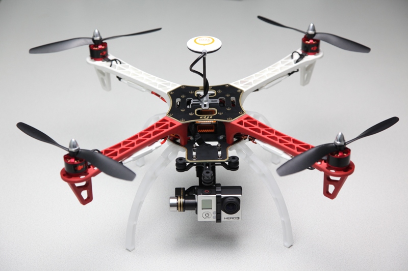
The Flamewheel f450

Sensor fusion

Sensor fusion is the combination of sensory data or data derived from disparate sources such that the resulting information has less uncertainty than what would be possible if these sources were to be used individually. In the context of drones, it is very useful because it enables us to combine many imprecise sensor measurements to form a more precise one like having precise positioning from 2 less precise GPS (dual GPS setting). It can also allows us to combine sensors with different sampling rates: typically, precise sensors with low sampling rate and less precise sensors with high sampling rates. Both cases will be relevant here.

A fundamental explanation of why this is possible at all comes from the central limit theorem: one sample from a distribution with a low variance is as good as n samples from a distribution with variance \(n\) times higher.

\[\mathbb{V}(X_i)=\sigma^2 ~~~~~ \mathbb{E}(X_i) = \mu\] \[\bar{X} = \frac{1}{n}\sum X_i\] \[\mathbb{V}(\bar{X}) = \frac{\sigma^2}{n} ~~~~~ \mathbb{E}(\bar{X}) = \mu\]

Notes on notation and conventions

The referential by default is the fixed world frame.

• \(\mathbf{x}\) designates a vector
• \(x_t\) is the random variable x at time t
• \(x_{t1:t2}\) is the product of the random variable x between t1 included and t2 included
• \(x^{(i)}\) designates the random variable x of the arbitrary particle i
• \(\hat{x}\) designates an estimated variable

POSE

POSE is the task of estimating the position and orientation of an object through time. It is a subroutine of Software Localization And Mapping (SLAM). We can formalize the problem as:

At each timestep, find the best expectation of a function of the hidden variable state (position and orientation), from their initial distribution and the history of observable random variables (such as sensor measurements).

• The state \(\mathbf{x}\)
• The function \(g(\mathbf{x})\) such that \(g(\mathbf{x}_t) = (\mathbf{p}_t, \mathbf{q}_t)\) where \(\mathbf{p}\) is the position and \(\mathbf{q}\) is the attitude as a quaternion.
• The observable variable \(\mathbf{y}\) composed of the sensor measurements \(\mathbf{z}\) and the control input \(\mathbf{u}\)

The algorithm inputs are:

• control inputs \(\mathbf{u}_t\) (the commands sent to the flight controller)
• sensor measurements \(\mathbf{z}_t\) coming from different sensors with different sampling rate
• information about the sensors (sensor measurements biases and matrix of covariance)

Trajectory data generation

The difficulties with using real flight data is that you need to get the true trajectory and you need enough data to check the efficiency of the filters.

To avoid these issues, the flight data is simulated through a model of trajectory generation from [1]. Data generated this way is called synthetic data. The algorithm inputs are the motion primitives defined by the quadcopter’s initial state, the desired motion duration, and any combination of components of the quadcopter’s position, velocity and acceleration at the motion’s end. The algorithm is essentially a closed form solution for the given primitives. The closed form solution minimizes a cost function related to the input aggressiveness.

The bulk of the method is that a differential equation representing the difference of position, velocity and acceleration between the starting and ending state is solved with the Pontryagin’s minimum principle using the appropriate Hamiltonian. Then, from that closed form solution, a per-axis cost can be calculated to pick the “least aggressive” trajectory out of different candidates. Finally, the feasibility of the trajectory is computed using the constraints of maximum thrust and body rate (angular velocity) limits.

For the purpose of this work, a scala implementation of the model was written. Then, some keypoints containing Gaussian components for the position, velocity acceleration, and duration were tried until a feasible set of keypoints was found. This method of data generation is both fast and a good enough approximation of the actual trajectories that a drone would perform in the real world.

Visualization of an example of a synthetic generated flight trajectory

Quaternion

Quaternions are extensions of complex numbers with 3 imaginary parts. Unit quaternions can be used to represent orientation, also referred to as attitude. Quaternions algebra make rotation composition simple and quaternions avoid the issue of gimbal lock.³ In all filters presented, quaternions represent the attitude.

\[\mathbf{q} = (q.r, q.i, q.j, q.k)^t = (q.r, \boldsymbol{\varrho})^T\]

Quaternion rotations composition is: \(q_2 q_1\) which results in \(q_1\) being rotated by the rotation represented by \(q_2\). From this, we can deduce that angular velocity integrated over time is simply \(q^t\) if \(q\) is the local quaternion rotation by unit of time. The product of two quaternions (also called Hamilton product) is computable by regrouping the same type of imaginary and real components together and accordingly to the identity:

\[i^2=j^2=k^2=ijk=-1\]

Rotation of a vector by a quaternion is done by: \(q v q^*\) where \(q\) is the quaternion representing the rotation, \(q^*\) its conjugate and \(v\) the vector to be rotated. The conjugate of a quaternion is:

\[q^* = - \frac{1}{2} (q + iqi + jqj + kqk)\]

The distance of between two quaternions, useful as an error metric is defined by the squared Frobenius norms of attitude matrix differences [2].

\[\| A(\mathbf{q}_1) - A(\mathbf{q}_2) \|^2_F = 6 - 2 Tr [ A(\mathbf{q}_1)A^t(\mathbf{q}_2) ]\]

where

\[A(\mathbf{q}) = (q.r^2 - \| \boldsymbol{\varrho} \|^2) I_{3 \times 3} + 2\boldsymbol{\varrho} \boldsymbol{\varrho}^T - 2q.r[\boldsymbol{\varrho} \times]\]

\[[\boldsymbol{\varrho} \times] = \left( \begin{array}{ccc} 0 & -q.k & q.j \\ q.k & 0 & -q.i \\ -q.j & q.i & 0 \\ \end{array} \right)\]

Helper functions and matrices

We introduce some helper matrices.

• \(\mathbf{R}_{b2f}\{\mathbf{q}\}\) is the body to fixed vector rotation matrix. It transforms vector in the body frame to the fixed world frame. It takes as parameter the attitude \(\mathbf{q}\).
• \(\mathbf{R}_{f2b}\{\mathbf{q}\}\) is its inverse matrix (from fixed to body).
• \(\mathbf{T}_{2a} = (0, 0, 1/m)^T\) is the scaling from thrust to acceleration (by dividing by the weight of the drone: \(\mathbf{F} = m\mathbf{a} \Rightarrow \mathbf{a} = \mathbf{F}/m)\) and then multiplying by a unit vector \((0, 0, 1)\)
• \[R2Q(\boldsymbol{\theta}) = (\cos(\| \boldsymbol{\theta} \| / 2), \sin(\| \boldsymbol{\theta} \| / 2) \frac{\boldsymbol{\theta}}{\| \boldsymbol{\theta} \|} )\] is a function that convert from a local rotation vector \(\boldsymbol{\theta}\) to a local quaternion rotation. The definition of this function come from converting \(\boldsymbol{\theta}\) to a body-axis angle, and then to a quaternion.
• \[Q2R(\mathbf{q}) = (q.i*s, q.j*s, q.k*s) \] is its inverse function where \(n = \arccos(q.w)*2\) and \(s = n/\sin(n/2)\)
• \(\Delta t\) is the lapse of time between t and the next tick (t+1)

Model

The drone is assumed to have rigid-body physics. It is submitted to the gravity and its own inertia. A rigid body is a solid body in which deformation is zero or so small it can be neglected. The distance between any two given points on a rigid body remains constant in time regardless of external forces exerted on it. This enables us to summarize the forces from the rotor as a thrust oriented in the direction normal to the plane formed by the 4 rotors, and an angular velocity.

Those variables are sufficient to describe the evolution of our drone with rigid-body physics:

• \(\mathbf{a}\) the total acceleration in the fixed world frame
• \(\mathbf{v}\) the velocity in the fixed world frame
• \(\mathbf{p}\) the position in the fixed world frame
• \(\boldsymbol{\omega}\) the angular velocity
• \(\mathbf{q}\) the attitude in the fixed world frame

Sensors

The sensors at the drone’s disposition are:

• Accelerometer: It generates \(\mathbf{a_A}\) a measurement of the total acceleration in the body frame referential the drone is submitted to at a high sampling rate. If the object is submitted to no acceleration then the accelerometer measure the earth’s gravity field. From that information, it could be possible to retrieve the attitude. Unfortunately, we are in a highly dynamic setting. Thus, it is possible when we can subtract the drone’s acceleration from the thrust to the total acceleration. This would require to know exactly the force exerted by the rotors at each instant. In this work, we assume that doing that separation, while being theoretically possible, is too impractical. The measurements model is: \[\mathbf{a_A}(t) = \mathbf{R}_{f2b}\{\mathbf{q}(t)\}\mathbf{a}(t) + \mathbf{a_A}^\epsilon\] where the covariance matrix of the noise of the accelerometer is \({\mathbf{R}_{\mathbf{a_A}}}_{3 \times 3}\) and \[\mathbf{a_A}^\epsilon \sim \mathcal{N}(\mathbf{0}, \mathbf{R}_{\mathbf{a_A}})\].

• Gyroscope:It generates \(\mathbf{\boldsymbol{\omega}_G}\) a measurement of the angular velocity in the body frame of the drone at the last timestep at a high sampling rate. The measurement model is: \[\mathbf{\boldsymbol{\omega}_G}(t) = \boldsymbol{\omega} + \mathbf{\boldsymbol{\omega}_G}^\epsilon\] where the covariance matrix of the noise of the accelerometer is \({\mathbf{R}_{\mathbf{\boldsymbol{\omega}_G}}}_{3 \times 3}\) and \[\mathbf{\boldsymbol{\omega}_G}^\epsilon_t \sim \mathcal{N}(\mathbf{0}, \mathbf{R}_{\mathbf{\boldsymbol{\omega}_G}})\].

• Position: It generates \(\mathbf{p_V}\) a measurement of the current position at a low sampling rate. This is usually provided by a Vicon (for indoor), GPS, a Tango or any other position sensor. The measurement model is: \[\mathbf{p_V}(t) = \mathbf{p}(t) + \mathbf{p_V}^\epsilon\] where the covariance matrix of the noise of the position is \({\mathbf{R}_{\mathbf{p_V}}}_{3 \times 3}\) and \[\mathbf{p_V}^\epsilon \sim \mathcal{N}(\mathbf{0}, \mathbf{R}_{\mathbf{p_V}})\].

• Attitude: It generates \(\mathbf{q_V}\) a measurement of the current attitude. This is usually provided in addition to the position by a Vicon or a Tango at a low sampling rate or the Magnemoter at a high sampling rate if the environment permits it (no high magnetic interference nearby like iron contamination). The magnetometer retrieves the attitude by assuming that the sensed magnetic field corresponds to the earth’s magnetic field. The measurement model is: \[\mathbf{q_V}(t) = \mathbf{q}(t)*R2Q(\mathbf{q_V}^\epsilon)\] where the \(3 \times 3\) covariance matrix of the noise of the attitude in radian before being converted by \(R2Q\) is \({\mathbf{R}_{\mathbf{q_V}}}_{3 \times 3}\) and \[\mathbf{q_V}^\epsilon \sim \mathcal{N}(\mathbf{0}, \mathbf{R}_{\mathbf{q_V}})\].

• Optical Flow: A camera that keeps track of the movement by comparing the difference of the position of some reference points. By using a companion distance sensor, it is able to retrieve the difference between the two perspective and thus the change in angle and position. \[\mathbf{dq_O}(t) = (\mathbf{q}(t-k)\mathbf{q}(t))*R2Q(\mathbf{dq_O}^\epsilon)\] \[\mathbf{dp_O}(t) = (\mathbf{p}(t) - \mathbf{p}(t-k)) + \mathbf{dp_O}^\epsilon\]

where the \(3 \times 3\) covariance matrix of the noise of the attitude variation in radian before being converted by \(R2Q\) is \({\mathbf{R}_{\mathbf{dq_O}}}_{3 \times 3}\) and \[\mathbf{dq_O}^\epsilon \sim \mathcal{N}(\mathbf{0}, \mathbf{R}_{\mathbf{dq_O}})\] and the position variation covariance matrix \({\mathbf{R}_{\mathbf{dp_O}}}_{3 \times 3}\) and \[\mathbf{dp_O}^\epsilon \sim \mathcal{N}(\mathbf{0}, \mathbf{R}_{\mathbf{dp_O}})\].

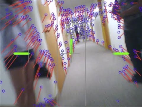
Optical flow from a moving drone

The notable difference with the position or attitude sensor is that the optical flow sensor, like the IMU, only captures time variation, not absolute values.

• Altimeter: An altimeter is a sensor that measure the altitude of the drone. For instance a LIDAR measure the time for the laser wave to reflect on a surface that is assumed to be the ground. A smart strategy is to only use the altimeter which is oriented with a low angle to the earth, else you also have to account that angle in the estimation of the altitude. \[z_A(t) = \sin(\text{pitch}(\mathbf{q(t)}))(\mathbf{p}(t).z + z_A^\epsilon)\] \({R_{z_A}}_{3 \times 3}\) and \[z_A^\epsilon \sim \mathcal{N}(0, R_{z_A})\]

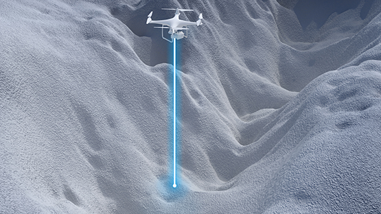
Rendering of the LIDAR laser of an altimeter

Some sensors are more relevant indoor and some others outdoor:

• Indoor: The sensors available indoor are the accelerometer, the gyroscope and the Vicon. The Vicon is a system composed of many sensors around a room that is able to track very accurately the position and orientation a mobile object. One issue with relying solely on the Vicon is that the sampling rate is low.

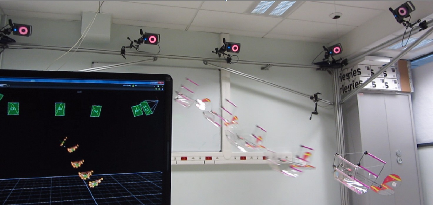
A Vicon setup

• Outdoor: The sensors available outdoor are the accelerometer, the gyroscope, the magnetometer, two GPS, an optical flow and an altimeter.

We assume that since the biases of the sensor could be known prior to the flight, both the sensor output measurements have been calibrated with no bias. Some filters like the ekf2 of the px4 flight stack keep track of the sensor biases but this is a state augmentation that was not deemed worthwhile.

Control inputs

Observations from the control input are not strictly speaking measurements but input of the state-transition model. The IMU is a sensor, thus strictly speaking, its measurements are not control inputs. However, in the literature, it is standard to use its measurements as control inputs. One of the advantage is that the IMU measures exactly the data we need for a prediction through the model dynamic. If we used instead a transformation of the thrust sent as command to the rotors, we would have to account for the rotors imprecision, the wind and other disturbances. Another advantage is that since the IMU has very high sampling rate, we can update very frequently the state with new transitions. The drawback is that the accelerometer is noisy. Fortunately, we can take into account the noise as a process model noise.

The control inputs at disposition are:

• Acceleration: \(\mathbf{a_A}_t\) from the acceloremeter
• Angular velocity: \(\mathbf{\boldsymbol{\omega}_G}_t\) from the gyroscope.

Model dynamic

• \(\mathbf{a}(t+1) = \mathbf{R}_{b2f}\{\mathbf{q}(t+1)\}(\mathbf{a_A}_t + \mathbf{a_A}^\epsilon_t)\) where \(\mathbf{a}^\epsilon_t \sim \mathcal{N}(\mathbf{0}, \mathbf{Q}_{\mathbf{a}_t })\)
• \(\mathbf{v}(t+1) = \mathbf{v}(t) + \Delta t \mathbf{a}(t) + \mathbf{v}^\epsilon_t\) where \(\mathbf{v}^\epsilon_t \sim \mathcal{N}(\mathbf{0}, \mathbf{Q}_{\mathbf{v}_t })\)
• \(\mathbf{p}(t+1) = \mathbf{p}(t) + \Delta t \mathbf{v}(t) + \mathbf{p}^\epsilon_t\) where \(\mathbf{p}^\epsilon_t \sim \mathcal{N}(\mathbf{0}, \mathbf{Q}_{\mathbf{p}_t })\)
• \(\boldsymbol{\omega}(t+1) = \mathbf{\boldsymbol{\omega}_G}_t + \mathbf{\boldsymbol{\omega}_G}^\epsilon_t\) where \(\mathbf{p}^\epsilon_t \sim \mathcal{N}(\mathbf{0}, \mathbf{Q}_{\mathbf{\boldsymbol{\omega}_G}_t })\)
• \(\mathbf{q}(t+1) = \mathbf{q}(t)*R2Q(\Delta t \boldsymbol{ \omega(t) })\)

Note that in our model, \(\mathbf{q}(t+1)\) must be known. Fortunately, as we will see later, our Rao-Blackwellized Particle Filter is conditioned under the attitude so it is known.

State

The time series of the variables of our dynamic model constitute a hidden Markov chain. Indeed, the model is “memoryless” and depends only on the current state and a sampled transition.

States contain variables that enable us to keep track of some of those hidden variables which is our ultimate goal (for POSE \(\mathbf{p}\) and \(\mathbf{q}\)). States at time \(t\) are denoted by \(\mathbf{x}_t\). Different filters require different state variables depending on their structure and assumptions.

Observation

Observations are revealed variables conditioned under the variables of our dynamic model. Our ultimate goal is to deduce the states from the observations.

Observations contain the control input \(\mathbf{u}\) and the measurements \(\mathbf{z}\).

\[\mathbf{y}_t = (\mathbf{z}_t, \mathbf{u}_t)^T = (\mathbf{p_V}_t, \mathbf{q_V}_t), ({t_C}_t, \mathbf{\boldsymbol{\omega}_C}_t))^T\]

Filtering and smoothing

Smoothing is the statistical task of finding the expectation of the state variable from the past history of observations and multiple observation variables ahead

\[\mathbb{E}[g(\mathbf{x}_{0:t}) | \mathbf{y}_{1:t+k}]\]

Which expand to,

\[\mathbb{E}[(\mathbf{p}_{0:t}, \mathbf{q}_{0:t}) | (\mathbf{z}_{1:t+k}, \mathbf{u}_{1:t+k})]\]

\(k\) is a contant and the first observation is \(y_1\)

Filtering is a kind of smoothing where you only have at disposal the current observation variable (\(k=0\))

Complementary Filter

The complementary filter is the simplest of all filters and is commonly used to retrieve the attitude because of its low computational complexity. The gyroscope and accelerometer both provide a measurement that can help us to estimate the attitude. Indeed, the gyroscope reads noisy measurement of the angular velocity from which we can retrieve the new attitude from the past one by time integration: \(\mathbf{q}_t = \mathbf{q}_{t-1}*R2Q(\Delta t \mathbf{\omega})\).

This is commonly called “Dead reckoning”⁴ and is prone to accumulation error, referred to as drift. Indeed, like Brownian motions, even if the process is unbiased, the variance grows with time. Reducing the noise cannot solve the issue entirely: even with extremely precise instruments, you are subject to floating-point errors.

Fortunately, even though the accelerometer gives us a highly noisy (vibrations, wind, etc … ) measurement of the orientation, it is not impacted by the effects of drifting because it does not rely on accumulation. Indeed, if not subject to other accelerations, the accelerometer measures the gravity field orientation. Since this field is oriented toward earth, it is possible to retrieve the current rotation from that field and by extension the attitude. However, a drone is under the influence of continuous and significant acceleration and vibration. Hence, the assumption that we retrieve the gravity field directly is wrong. Nevertheless, we could solve this by subtracting the acceleration deduced from the thrust control input. It is unpractical so this approach is not pursued in this work, but understanding this filter is still useful.

The idea of the filter itself is to combine the precise “short-term” measurements of the gyroscope subject to drift with the “long-term” measurements of the accelerometer.

State

This filter is very simple. The only requirement is that the last estimated attitude must be stored along with its timestamp in order to calculate \(\Delta t\). \[\mathbf{x}_t = \mathbf{q}_t\] \[\hat{\mathbf{q}}_{t+1} = \alpha (\hat{\mathbf{q}}_t + \Delta t \mathbf{\omega}_t) + (1 - \alpha) {\mathbf{q_A}}_{t+1}\] \(\alpha \in [0, 1]\). Usually, \(\alpha\) is set to a high-value like \(0.98\). It is very intuitive to see why this should approximately “work”, the data from the accelerometer continuously corrects the drift from the gyroscope.

┌──────┐ ┌───────────────────────────────────────────┐                         
│      │ │                                           │                         
│      │<┘┌───────────────────────────┐  ┌────────┐  │                         
│      ├──┘                           │  │        │  │ ┌─────────┐             
│Buffer│     ┌─────┐    ┌───────┐     └─>│        │  │ │         │             
│      │     │     │    │       │        │Rotation│  │ │         │  ┌─────────┐
│      ├────>│     ├───>│BR2Quat├───────>│        │  └─┤         │  │         │
│      │     │Integ│    │       │        │        ├───>│Combining├─>│Block out│
└──────┘  ┌─>│     │    └───────┘        └────────┘    │         │  │         │
          │  │     │                                ┌─>│         │  └─────────┘
┌───────┐ │  └─────┘┌────────────────┐   ┌────────┐ │  │         │             
│       │ │         │                │   │        │ │  └─────────┘             
│       ├─┘         │┌─────────────┐ └──>│        │ │                          
│Map IMU├───────────┘│             │     │ACC2Quat├─┘                          
│       │            │Map CI Thrust├────>│        │                            
│       │            │             │     │        │                            
└───────┘            └─────────────┘     └────────┘                            

Complementary Filter graph structure

Figure 9 is the plot of the distance from the true quaternion after 15s of an arbitrary trajectory when \(\alpha = 1.0\) meaning that the accelerometer does not correct the drift.

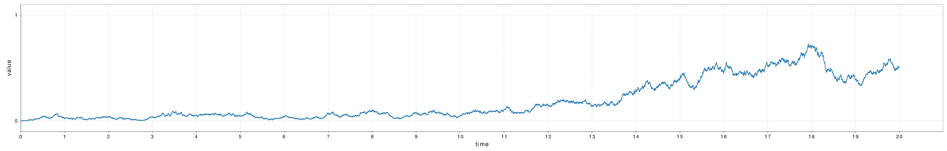
CF with alpha = 1.0

Figure 10 is that same trajectory with \(\alpha = 0.98\).

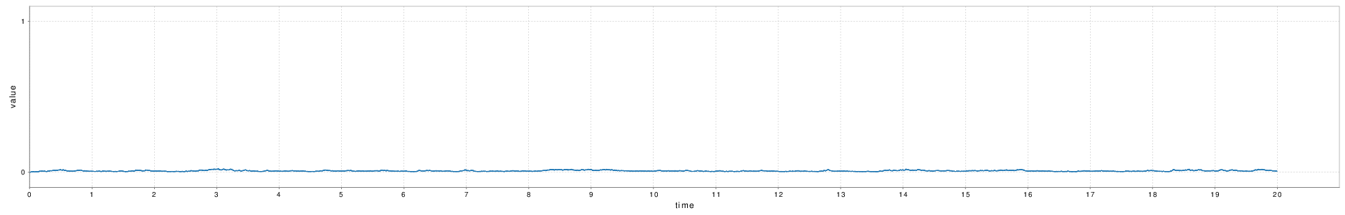
CF with alpha = 0.98

We can observe here the long-term importance of being able to correct the drift, even if ever so slightly at each timestep.

Asynchronous Augmented Complementary Filter

As explained previously, in this highly-dynamic setting, combining the gyroscope and the accelerometer to retrieve the attitude is not satisfactory. However, we can reuse the intuition from the complementary filter, which is to combine precise but drifting short-term measurements to other measurements that do not suffer from drifting. This enables a simple and computationally inexpensive novel filter that we will be able to use later as a baseline. In this context, the short-term measurements are the acceleration and angular velocity from the IMU, and the non-drifting measurements are the position and attitude from the Vicon.

We will also add the property that the data from the sensors are asynchronous. As with all following filters, we deal with asynchronicity by updating the state to the most likely state so far for any new sensor measurement incoming. This is a consequence of the sensors having different sampling rate.

• IMU update \[\mathbf{v}_t = \mathbf{v}_{t-1} + \Delta t_v \mathbf{a_A}_t\] \[\boldsymbol{\omega}_t = \boldsymbol{\mathbf{\omega_G}}_t\] \[\mathbf{p}_t = \mathbf{p}_{t-1} + \Delta t \mathbf{v}_{t-1}\] \[\mathbf{q}_t = \mathbf{q}_{t-1}R2Q(\Delta t \boldsymbol{\omega}_{t-1})\]

• Vicon update \[\mathbf{p}_t = \alpha \mathbf{p_V} + (1 - \alpha) (\mathbf{p}_{t-1} + \Delta t \mathbf{v}_{t-1})\] \[\mathbf{q}_t = \alpha \mathbf{q_V} + (1 - \alpha) (\mathbf{q}_{t-1}R2Q(\Delta t \boldsymbol{\omega}_{t-1}))\]

State

The state has to be more complex because the filter now estimates both the position and the attitude. Furthermore, because of asynchronicity, we have to store the last angular velocity, the last linear velocity, and the last time the linear velocity has been updated (to retrieve \(\Delta t_v = t - t_a\) where \(t_a\) is the last time we had an update from the accelerometer).

\[\mathbf{x}_t = (\mathbf{p}_t, \mathbf{q}_t, \boldsymbol{\omega}_t, \mathbf{a}_t, t_a)\]

The structure of this filter and all of the filters presented thereafter is as follow:

 ┌───────┐                          ┌──────┐   ┌─────┐  ┌─────────┐
 │       │                          │      │   │     │  │         │
 │Map IMU├─┐   ┌─────┐  ┌───────┐   │      ├──>│P & Q├─>│Block out│
 │       │ │   │     │  │       ├──>│Update│   │     │  │         │
 └───────┘ └──>│     │  │       │   │      ├─┐ └─────┘  └─────────┘
               │Merge├─>│ZipLast│   │      │ │                     
┌─────────┐ ┌─>│     │  │       │<┐ └──────┘ │           ┌──────┐  
│         │ │  │     │  │       │ │          │           │      │  
│Map Vicon├─┘  └─────┘  └───────┘ │          │           │      │  
│         │                       │          └──────────>│Buffer│  
└─────────┘                       └──────────────────────┤      │  
                                                         │      │  
                                                         └──────┘  

A graph of the filters structure in scala-flow

Kalman Filter

Bayesian inference

Bayesian inference is a method of statistical inference in which Bayes’ theorem is used to update the probability for a hypothesis when more evidence or information becomes available. In this Bayes setting, the prior is the estimated distribution of the previous state at time \(t-1\), the likelihood correspond to the likelihood of getting the new data from the sensor given the prior and finally, the posterior is the updated estimated distribution.

Model

The Kalman filter requires that both the model process and the measurement process are linear gaussian. Linear gaussian processes are of the form: \[\mathbf{x}_t = f(\mathbf{x}_{t-1}) + \mathbf{w}_t\] where \(f\) is a linear function and \(\mathbf{w}_t\) a gaussian process: it is sampled from an arbitrary gaussian distribution.

The Kalman filter is a direct application of bayesian inference. It combines the prediction of the distribution given the estimated prior state and the state-transition model.

\[\mathbf{x}_t = \mathbf{F}_t \mathbf{x}_{t-1} + \mathbf{B}_t \mathbf{u}_t + \mathbf{w}_t \]

• \(\mathbf{x}_t\) the state
• \(\mathbf{F}_t\) the state transition model
• \(\mathbf{B}_t\) the control-input model
• \(\mathbf{u}_t\) the control vector
• \(\mathbf{w}_t\) process noise drawn from \(\mathbf{w}_t \sim N(0, \mathbf{Q}_k)\)

and the estimated distribution given the data coming from the sensors.

\[\mathbf{y}_t = \mathbf{H}_t \mathbf{x}_{t} + \mathbf{v}_t \]

• \(\mathbf{y}_t\) measurements
• \(\mathbf{H}_t\) the state to measurement matrix
• \(\mathbf{w}_t\) measurement noise drawn from \(\mathbf{w}_t \sim N(0, \mathbf{R}_k)\)

Because, both the model process and the sensor process are assumed to be linear Gaussian, we can combine them into a Gaussian distribution. Indeed, the product of the distribution of two Gaussian forms a new Gaussian distribution.

\[P(\mathbf{x}_{t}) \propto P(\mathbf{x}^{-}_{t}|\mathbf{x}_{t-1}) \cdot P(\mathbf{x}_t | \mathbf{y}_t )\] \[\mathcal{N}(\mathbf{x}_{t}) \propto \mathcal{N}(\mathbf{x}^{-}_{t}|\mathbf{x}_{t-1}) \cdot \mathcal{N}(\mathbf{x}_t | \mathbf{y}_t )\]

where \(\mathbf{x}^{-}_{t}\) is the predicted state from the previous state and the state-transition model.

Kalman filter keeps track of the parameters of that gaussian: the mean state and the covariance of the state which represents the uncertainty about our last prediction. The mean of that distribution is also the best current state estimation of the filter.

By keeping track of the uncertainty, we can optimally combine the normals by knowing what importance to give to the difference between the expected sensor data and the actual sensor data. That factor is the Kalman gain.

• predict:
  • predicted state: \(\hat{\mathbf{x}}^{-}_t = \mathbf{F}_t \mathbf{x}_{t-1} + \mathbf{B}_t \mathbf{u}_t\)
  • predicted covariance: \(\mathbf{\Sigma}^{-}_t = \mathbf{F}_{t-1} \mathbf{\Sigma}^{-}_{t-1} \mathbf{F}_{t-1}^T + \mathbf{Q}_t\)
• update:
  • predicted measurements: \(\hat{\mathbf{z}} = \mathbf{H}_t \hat{\mathbf{x}}^{-}_t\)
  • innovation: \((\mathbf{z}_t - \hat{\mathbf{z}})\)
  • innovation covariance: \(\mathbf{S} = \mathbf{H}_t \mathbf{\Sigma}^{-}_t \mathbf{H}_t^T + \mathbf{R}_t\)
  • optimal kalman gain: \(\mathbf{K} = \mathbf{\Sigma}^{-}_t \mathbf{H}_t^T \mathbf{S}^{-1}\)
  • updated state: \(\mathbf{\Sigma}_t = \mathbf{\Sigma}^-_t + \mathbf{K} \mathbf{S} \mathbf{K}^T\)
  • updated covariance: \(\hat{\mathbf{x}}_t = \hat{\mathbf{x}}^{-}_t + \mathbf{K}(\mathbf{z}_t - \hat{\mathbf{z}})\)

Asynchronous Kalman Filter

It is not necessary to apply the full Kalman update at each measurement. Indeed, \(\mathbf{H}\) can be sliced to correspond to the measurements currently available.

To be truly asynchronous, you also have to account for the different sampling rates. There are two cases :

• The required data for the update step (the control inputs) can arrive multiple times before any of the data of the update step (the measurements) occur.
• Inversely, it is possible that the measurements occur at a higher sampling rate than the control inputs.

The strategy chosen here is as follows:

1. Multiple prediction steps without any update step may happen without making the algorithm inconsistent.
2. An update is always immediately preceded by a prediction step. This is a consequence of the requirement that the innovation must measure the difference between the predicted measurement from the state at the exact current time and the measurements. Thus, if the measurements are not synchronized with the control inputs, use the most likely control input for the prediction step. Repeating the last control input was the method used for the accelerometer and the gyroscope data as control input.

Extended Kalman Filters

In the previous section, we have shown that the Kalman Filter is only applicable when both the process model and the measurement model are linear Gaussian processes.

• The noise of the measurements and of the state-transition must be Gaussian
• The state-transition function and the measurement to state function must be linear.

Furthermore, it is provable that Kalman filters are optimal linear filters.

However, in our context, one component of the state, the attitude, is intrinsically non-linear. Indeed, rotations and attitudes belong to \(SO(3)\) which is not a vector space. Therefore, we cannot use vanilla Kalman filters. The filters that we present thereafter relax those requirements.

One example of such extension is the extended Kalman filter (EKF) that we will present here. The EKF relax the linearity requirement by using differentiation to calculate an approximation of the first order of the functions required to be linear. Our state transition function and measurement function can now be expressed in the free forms \(f(\mathbf{x}_t)\) and \(h(\mathbf{x}_t)\) and we define the matrix \(\mathbf{F}_t\) and \(\mathbf{H}_t\) as their Jacobian.

\[{\mathbf{F}_t}_{10 \times 10} = \left . \frac{\partial f}{\partial \mathbf{x} } \right \vert _{\hat{\mathbf{x}}_{t-1},\mathbf{u}_{t-1}}\]

\[{\mathbf{H}_t}_{7 \times 7} = \left . \frac{\partial h}{\partial \mathbf{x} } \right \vert _{\hat{\mathbf{x}}_{t}}\]

• predict:
  • predicted state: \(\hat{\mathbf{x}}^{-}_t = f(\mathbf{x}_{t-1}) + \mathbf{B}_t \mathbf{u}_t\)
  • predicted covariance: \(\mathbf{\Sigma}^{-}_t = \mathbf{F}_{t-1} \mathbf{\Sigma}^{-}_{t-1} \mathbf{F}_{t-1}^T + \mathbf{Q}_t\)
• update:
  • predicted measurements: \(\hat{\mathbf{z}} = h(\hat{\mathbf{x}}^{-}_t)\)
  • innovation: \((\mathbf{z}_t - \hat{\mathbf{z}})\)
  • innovation covariance: \(\mathbf{S} = \mathbf{H}_t \mathbf{\Sigma}^{-}_t \mathbf{H}_t^T + \mathbf{R}_t\)
  • optimal kalman gain: \(\mathbf{K} = \mathbf{\Sigma}^{-}_t \mathbf{H}_t^T \mathbf{S}^{-1}\)
  • updated state: \(\mathbf{\Sigma}_t = \mathbf{\Sigma}^-_t + \mathbf{K} \mathbf{S} \mathbf{K}^T\)
  • updated covariance: \(\hat{\mathbf{x}}_t = \hat{\mathbf{x}}^{-}_t + \mathbf{K}(\mathbf{z}_t - \hat{\mathbf{z}})\)

EKF for POSE

State

For the EKF, we will use the following state:

\[\mathbf{x}_t = (\mathbf{v}_t, \mathbf{p}_t, \mathbf{q}_t)^T\]

Initial state \(\mathbf{x}_0\) at \((\mathbf{0}, \mathbf{0}, (1, 0, 0, 0))\)

Indoor Measurements model

1. Position: \[\mathbf{p_V}(t) = \mathbf{p}(t)^{(i)} + \mathbf{p_V}^\epsilon_t\] where \(\mathbf{p_V}^\epsilon_t \sim \mathcal{N}(\mathbf{0}, \mathbf{R}_{\mathbf{p_V}_t })\)
2. Attitude: \[\mathbf{q_V}(t) = \mathbf{q}(t)^{(i)}*R2Q(\mathbf{q_V}^\epsilon_t)\] where \(\mathbf{q_V}^\epsilon_t \sim \mathcal{N}(\mathbf{0}, \mathbf{R}_{\mathbf{q_V}_t })\)

Kalman prediction

The model dynamic defines the following model, state-transition function \(f(\mathbf{x}, \mathbf{u})\) and process noise \(\mathbf{w}\) with covariance matrix \(\mathbf{Q}\)

\[\mathbf{x}_t = f(\mathbf{x}_{t-1}, \mathbf{u}_t) + \mathbf{w}_t\]

\[f((\mathbf{v}, \mathbf{p}, \mathbf{q}), (\mathbf{a_A}, \mathbf{\boldsymbol{\omega}_G})) = \left( \begin{array}{c} \mathbf{v} + \Delta t \mathbf{R}_{b2f}\{\mathbf{q}_{t-1}\} \mathbf{a} \\ \mathbf{p} + \Delta t \mathbf{v} \\ \mathbf{q}*R2Q({\Delta t} \boldsymbol{\omega}_G) \end{array} \right)\]

Now, we need to derive the jacobian of \(f\). We will use sagemath to retrieve the 28 relevant different partial derivatives of \(q\).

\[{\mathbf{F}_t}_{10 \times 10} = \left . \frac{\partial f}{\partial \mathbf{x} } \right \vert _{\hat{\mathbf{x}}_{t-1},\mathbf{u}_{t-1}}\]

\[\hat{\mathbf{x}}^{-(i)}_t = f(\mathbf{x}^{(i)}_{t-1}, \mathbf{u}_t)\] \[\mathbf{\Sigma}^{-(i)}_t = \mathbf{F}_{t-1} \mathbf{\Sigma}^{-(i)}_{t-1} \mathbf{F}_{t-1}^T + \mathbf{Q}_t\]

Kalman measurements update

\[\mathbf{z}_t = h(\mathbf{x}_t) + \mathbf{v}_t\]

The measurement model defines \(h(\mathbf{x})\)

\[\left( \begin{array}{c} \mathbf{p_V}\\ \mathbf{q_V}\\ \end{array} \right) = h((\mathbf{v}, \mathbf{p}, \mathbf{q})) = \left( \begin{array}{c} \mathbf{p}\\ \mathbf{q}\\ \end{array} \right)\]

The only complex partial derivatives to calculate are the ones of the acceleration, because they have to be rotated first. Once again, we use sagemath: \(\mathbf{H_a}\) is defined by the script in the appendix B.

\[{\mathbf{H}_t}_{10 \times 7} = \left . \frac{\partial h}{\partial \mathbf{x} } \right \vert _{\hat{\mathbf{x}}_{t}} = \left( \begin{array}{ccc} \mathbf{0}_{3 \times 3} & & \\ & \mathbf{I}_{3 \times 3} & \\ & & \mathbf{I}_{4 \times 4}\\ \end{array} \right)\]

\[{\mathbf{R}_t}_{7 \times 7} = \left( \begin{array}{cc} \mathbf{R}_{\mathbf{p_V}} & \\ & {\mathbf{R}'_{\mathbf{q_V}}}_{4 \times 4}\\ \end{array} \right)\]

\(\mathbf{R}'_{\mathbf{q_V}}\) has to be \(4 \times 4\) and has to represent the covariance of the quaternion. However, the actual covariance matrix \(\mathbf{R}_{\mathbf{q_V}}\) is \(3 \times 3\) and represent the noise in terms of a rotation vector around the x, y, z axes.

We transform this rotation vector into a quaternion using our function \(R2Q\). We can compute the new covariance matrix \(\mathbf{R}'_{\mathbf{q_V}}\) using Unscented Transform.

Unscented Transform

The unscented transform (UT) is a mathematical function used to estimate statistics after applying a given nonlinear transformation to a probability distribution. The idea is to use points that are representative of the original distribution, sigma points. We apply the transformation to those sigma points and calculate new statistics using the transformed sigma points. The sigma points must have the same mean and covariance as the original distribution.

The minimal set of symmetric sigma points can be found using the covariance of the initial distribution. The \(2N + 1\) minimal symmetric set of sigma points are the mean and the set of points corresponding to the mean plus and minus one of the direction corresponding to the covariance matrix. In one dimension, the square root of the variance is enough. In N-dimensions, you must use the Cholesky decomposition of the covariance matrix. The Cholesky decomposition finds the matrix \(L\) such that \(\Sigma = LL^t\).

Unscented tranformation

Kalman update

\[\mathbf{S} = \mathbf{H}_t \mathbf{\Sigma}^{-}_t \mathbf{H}_t^T + \mathbf{R}_t\] \[\hat{\mathbf{z}} = h(\hat{\mathbf{x}}^{-}_t)\] \[\mathbf{K} = \mathbf{\Sigma}^{-}_t \mathbf{H}_t^T \mathbf{S}^{-1}\] \[\mathbf{\Sigma}_t = \mathbf{\Sigma}^-_t + \mathbf{K} \mathbf{S} \mathbf{K}^T\] \[\hat{\mathbf{x}}_t = \hat{\mathbf{x}}^{-}_t + \mathbf{K}(\mathbf{z}_t - \hat{\mathbf{z}})\]

F partial derivatives

Q.<i,j,k> = QuaternionAlgebra(SR, -1, -1)

var('q0, q1, q2, q3')
var('dt')
var('wx, wy, wz')

q = q0 + q1*i + q2*j + q3*k

w = vector([wx, wy, wz])*dt
w_norm = sqrt(w[0]^2 + w[1]^2 + w[2]^2)
ang = w_norm/2
w_normalized = w/w_norm
sin2 = sin(ang)
qd = cos(ang) + w_normalized[0]*sin2*i + w_normalized[1]*sin2*j 
	+ w_normalized[2]*sin2*k

nq = q*qd

v = vector(nq.coefficient_tuple())

for sym in [wx, wy, wz, q0, q1, q2, q3]:
    d = diff(v, sym)
    exps = map(lambda x: x.canonicalize_radical().full_simplify(), d)
    for i, e in enumerate(exps):
        print(sym, i, e) 
		

Unscented Kalman Filters

The EKF has three flaws in our case:

• The linearization gives an approximate form which result in approximation errors
• The prediction step of the EKF assumes that the linearized form of the transformation can capture all the information needed to apply the transformation to the gaussian distribution pre-transformation. Unfortunately, this is only true near the region of the mean. The transformation of the tail of the gaussian distribution may need to be very different.
• It attempts to define a Gaussian covariance matrix for the attitude quaternion. This does not make sense because it does not account for the requirement of the quaternion being in a 4 dimensional unit sphere.

The Unscented Kalman Filter (UKF) does not suffer from the two first flaws, but it is more computationally expensive as it requires a Cholesky factorisation that grows exponentially in complexity with the number of dimensions.

Indeed, the UKF applies an unscented transformation to sigma points of the current approximated distribution. The statistics of the new approximated Gaussian are found through this unscented transform. The EKF linearizes the transformation, the UKF approximates the resulting Gaussian after the transformation. Hence, the UKF can take into account the effects of the transformation away from the mean which might be drastically different.

The implementation of an UKF still suffers greatly from quaternions not belonging to a vector space. The approach taken by [3] is to use the error quaternion defined by \(\mathbf{e}_i = \mathbf{q}_i\bar{\mathbf{q}}\). This approach has the advantage that similar quaternion differences result in similar error. But apart from that, it does not have any profound justification. We must compute a sound average weighted quaternion of all sigma points. An algorithm is described in the following section.

Average quaternion

Unfortunately, the average of quaternions components \(\frac{1}{N} \sum q_i\) or barycentric mean is unsound: Indeed, attitudes do not belong to a vector space but a homogenous Riemannian manifold (the four dimensional unit sphere). To convince yourself of the unsoundness of the barycentric mean, see that the addition and barycentric mean of two unit quaternions is not necessarily a unit quaternion (\((1, 0, 0, 0)\) and \((-1, 0, 0, 0)\) for instance. Furthermore, angles being periodic, the barycentric mean of a quaternion with angle \(-178^\circ\) and another with same body-axis and angle \(180^\circ\) gives \(1^\circ\) instead of the expected \(-179^\circ\).

To calculate the average quaternion, we use an algorithm which minimizes a metric that corresponds to the weighted attitude difference to the average, namely the weighted sum of the squared Frobenius norms of attitude matrix differences.

\[\bar{\mathbf{q}} = arg \min_{q \in \mathbb{S}^3} \sum w_i \| A(\mathbf{q}) - A(\mathbf{q}_i) \|^2_F\]

where \(\mathbb{S}^3\) denotes the unit sphere.

The attitude matrix \(A(\mathbf{q})\) and its corresponding Frobenius norm have been described in the quaternion section.

Intuition

The intuition of keeping track of multiple representatives of the distribution is exactly the approach taken by the particle filter. The particle filter has the advantage that the distribution is never transformed back to a gaussian so there are fewer assumptions made about the noise and the transformation. It is only required to be able to calculate the expectation from a weighted set of particles.

Particle Filter

Particle filters are computationally expensive. This is the reason why their usage is not very popular currently for low-powered embedded systems like drones. However, they are used in Avionics for planes since the computational resources are less scarce but precision crucial. Accelerating hardware could widen the usage of particle filters to embedded systems.

Particle filters are sequential Monte Carlo methods. Like all Monte Carlo methods, they rely on repeated sampling for estimation of a distribution.

Monte Carlo estimation of pi

The particle filter is itself a weighted particle representation of the posterior:

\[p(\mathbf{x}) = \sum w^{(i)}\delta(\mathbf{x} - \mathbf{x}^{(i)})\] where \(\delta\) is the dirac delta function. The dirac delta function is zero everywhere except at zero, with an integral of one over the entire real line. It represents here the ideal probability density of a particle.

Importance sampling

Weights are computed through importance sampling. With importance sampling, each particle does not equally represent the distribution. Importance sampling enables us to use sampling from another distribution to estimate properties from the target distribution of interest. In most cases, it can be used to focus sampling on a specific region of the distribution. In our case, by choosing the right importance distribution (the dynamics of the model as we will see later), we can re-weight particles based on the likelihood from the measurements (\(p(\mathbf{y} | \mathbf{x})\).

Importance sampling is based on the identity:

\[ \begin{aligned} \mathbb{E}[\mathbf{g}(\mathbf{x}) | \mathbf{y}_{1:T}] &= \int \mathbf{g}(\mathbf{x})p(\mathbf{x}|\mathbf{y}_{1:T})d\mathbf{x} \\ &= \int \left [\mathbf{g}(\mathbf{x})\frac{p(\mathbf{x}|\mathbf{y}_{1:T})}{\mathbf{\pi}(\mathbf{x}|\mathbf{y}_{1:T})} \right ] \mathbf{\pi}(\mathbf{x}|\mathbf{y}_{1:T}) d\mathbf{x} \end{aligned} \]

Thus, it can be approximated as \[ \begin{aligned} \mathbb{E}[\mathbf{g}(\mathbf{x}) | \mathbf{y}_{1:T}] &\approx \frac{1}{N} \sum_i^N \frac{p(\mathbf{x}^{(i)}|\mathbf{y}_{1:T})}{\mathbf{\pi}(\mathbf{x}^{(i)}|\mathbf{y}_{1:T})}\mathbf{g}(\mathbf{x}^{(i)}) &\approx \sum^N_i w^{(i)} \mathbf{g}(\mathbf{x}^{(i)}) \end{aligned} \]

where \(N\) samples of \(\mathbf{x}\) are drawn from the importance distribution \(\mathbf{\pi}(\mathbf{x}|\mathbf{y}_{1:T})\)

And the weights are defined as:

\[w^{(i)} = \frac{1}{N} \frac{p(\mathbf{x}^{(i)}|\mathbf{y}_{1:T})}{\mathbf{\pi}(\mathbf{x}^{(i)}|\mathbf{y}_{1:T})}\]

Computing \(p(\mathbf{x}^{(i)}|\mathbf{y}_{1:T}\) is hard (if not impossible), but fortunately we can compute the unnormalized weight instead:

\[w^{(i)}* = p(\mathbf{y}_{1:T}|\mathbf{x}^{(i)})p(\mathbf{x}^{(i))}{\mathbf{\pi}(\mathbf{x}^{(i)}|\mathbf{y}_{1:T})}\]

and normalizing it afterwards

\[\sum^N_i w^{(i)*} = 1 \Rightarrow w^{(i)} = \frac{w^{*(i)}}{\sum^N_j w^{*(i)}}\]

Sequential Importance Sampling

The last equation becomes more and more computationally expensive as T grows larger (the joint variable of the time series grows larger). Fortunately, Sequential Importance Sampling is an alternative recursive algorithm that has a fixed amount of computation at each iteration:

\[ \begin{aligned} p(\mathbf{x}_{0:k} | \mathbf{y}_{0:k}) &\propto p(\mathbf{y}_k | \mathbf{x}_{0:k}, \mathbf{y}_{1:k-1})p(\mathbf{x}_k | \mathbf{y}_{1:k-1}) \\ &\propto p(\mathbf{y}_k | \mathbf{x}_{k})p(\mathbf{x}_k | \mathbf{x}_{0:k-1}, \mathbf{y}_{1:k-1})p(\mathbf{x}_{0:k-1} | \mathbf{y}_{1:k-1}) \\ &\propto p(\mathbf{y}_k | \mathbf{x}_{k})p(\mathbf{x}_k | \mathbf{x}_{k-1})p(\mathbf{x}_{0:k-1} | \mathbf{y}_{1:k-1}) \end{aligned} \]

The importance distribution is such that \(\mathbf{x}^i_{0:k} \sim \pi(\mathbf{x}_{0:k} | \mathbf{y}_{1:k})\) with the according importance weight: \[w^{(i)}_k \propto \frac{p(\mathbf{y}_k | \mathbf{x}^{(i)}_{k})p(\mathbf{x}^{(i)}_k | \mathbf{x}^{(i)}_{k-1})p(\mathbf{x}^{(i)}_{0:k-1} | \mathbf{y}_{1:k-1})}{\pi(\mathbf{x}_{0:k} | \mathbf{y}_{1:k})}\]

We can express the importance distribution recursively: \[\pi(\mathbf{x}_{0:k} | \mathbf{y}_{1:k}) = \pi(\mathbf{x}_{k} |\mathbf{x}_{0:k-1}, \mathbf{y}_{1:k})\pi(\mathbf{x}_{0:k-1} | \mathbf{y}_{1:k-1})\]

The recursive structure propagates to the weight itself:

\[ \begin{aligned} w^{(i)}_k &\propto \frac{p(\mathbf{y}_k | \mathbf{x}^{(i)}_{k})p(\mathbf{x}^{(i)}_k | \mathbf{x}^{(i)}_{k-1})}{\pi(\mathbf{x}_{k} |\mathbf{x}_{0:k-1}, \mathbf{y}_{1:k})} \frac{p(\mathbf{x}^{(i)}_{0:k-1} | \mathbf{y}_{1:k-1})}{\pi(\mathbf{x}_{0:k-1} | \mathbf{y}_{1:k-1})} \\ &\propto \frac{p(\mathbf{y}_k | \mathbf{x}^{(i)}_{k})p(\mathbf{x}^{(i)}_k | \mathbf{x}^{(i)}_{k-1})}{\pi(\mathbf{x}_{k} |\mathbf{x}_{0:k-1}, \mathbf{y}_{1:k})} w^{(i)}_{k-1} \end{aligned} \]

We can further simplify the formula by choosing the importance distribution to be the dynamics of the model: \[\pi(\mathbf{x}_{k} |\mathbf{x}_{0:k-1}, \mathbf{y}_{1:k}) = p(\mathbf{x}^{(i)}_k | \mathbf{x}^{(i)}_{k-1})\] \[ w^{*(i)}_k = p(\mathbf{y}_k | \mathbf{x}^{(i)}_{k}) w^{(i)}_{k-1}\]

As previously, it is then only needed to normalize the resulting weight.

\[\sum^N_i w^{(i)*} = 1 \Rightarrow w^{(i)} = \frac{w^{*(i)}}{\sum^N_j w^{*(i)}}\]

Resampling

When the number of effective particles is too low (less than \(1/10\) of N having weight \(1/10\)), we apply systematic resampling. The idea behind resampling is simple. The distribution is represented by a number of particles with different weights. As time goes on, the repartition of weights degenerates. A large subset of particles end up having negligible weight which make them irrelevant and only a few particles represent most of the distribution. In the most extreme case, one particle represents the whole distribution.

To avoid that degeneration, when the weights are too unbalanced, we resample from the weights distribution: pick N times among the particle and assign them a weight of \(1/N\), each pick has odd \(w_i\) to pick the particle \(p_i\). Thus, some particles with large weights are split up into smaller clone particle and others with small weights are never picked. This process is remotely similar to evolution: at each generation, the most promising branch survives and replicate while the less promising dies off.

A popular method for resampling is systematic sampling as described by [4]:

Sample \(U_1 \sim \mathcal{U} [0, \frac{1}{N} ]\) and define \(U_i = U_1 + \frac{i-1 }{N}\) for \(i = 2, \ldots, N\)

Rao-Blackwellized Particle Filter

Introduction

Compared to a plain particle filter, RBPF leverages the linearity of some components of the state by assuming our model to be Gaussian conditioned on a latent variable: Given the attitude \(q_t\), our model is linear. This is where RBPF shines: We use particle filtering to estimate our latent variable, the attitude, and we use the optimal kalman filter to estimate the state variable. If a plain particle can be seen as the simple average of particle states, then the RBPF can be seen as the “average” of many Gaussians. Each particle is an optimal kalman filter conditioned on the particle’s latent variable, the attitude.

Indeed, the advantage of particle filters is that they assume no particular form for the posterior distribution and transformation of the state. But as the state widens in dimensions, the number of needed particles to keep a good estimation grows exponentially. This is a consequence of [“the curse of dimensionality”}(https://en.wikipedia.org/wiki/Curse_of_dimensionality): for each dimension, we would have to consider all additional combination of state components. In our context, we have 10 dimensions (\(\mathbf{v}\),\(\mathbf{p}\),\(\mathbf{q}\)), which is already large, and it would be computationally expensive to simulate a too large number of particles.

Kalman filters on the other hand do not suffer from such exponential growth, but as explained previously, they are inadequate for non-linear transformations. RBPF is the best of both worlds by combining a particle filter for the non-linear components of the state (the attitude) as a latent variable, and Kalman filters for the linear components of the state (velocity and position). For ease of notation, the linear component of the state will be referred to as the state and designated by \(\mathbf{x}\) even though the actual state we are concerned with should include the latent variable \(\boldsymbol{\theta}\).

Related work

Related work of this approach is [5]. However, it differs by:

• adapting the filter to drones by taking into account that the system is too dynamic for assuming that the accelerometer simply output the gravity vector. This is solved by augmenting the state with the acceleration as shown later.
• add an attitude sensor.

Latent variable

We introduce the latent variable \(\boldsymbol{\theta}\)

The latent variable \(\boldsymbol{\theta}\) has for sole component the attitude: \[\boldsymbol{\theta} = (\mathbf{q})\]

\(q_t\) is estimated from the product of the attitude of all particles \(\mathbf{\theta^{(i)}} = \mathbf{q}^{(i)}_t\) as the “average” quaternion \(\mathbf{q}_t = avgQuat(\mathbf{q}^n_t)\). \(x^n\) designates the product of all n arbitrary particle.

As stated in the previous section, The weight definition is:

\[w^{(i)}_t = \frac{p(\boldsymbol{\theta}^{(i)}_{0:t} | \mathbf{y}_{1:t})}{\pi(\boldsymbol{\theta}^{(i)}_{0:t} | \mathbf{y}_{1:t})}\]

From the definition and the previous section, it is provable that:

\[w^{(i)}_t \propto \frac{p(\mathbf{y}_t | \boldsymbol{\theta}^{(i)}_{0:t-1}, \mathbf{y}_{1:t-1})p(\boldsymbol{\theta}^{(i)}_t | \boldsymbol{\theta}^{(i)}_{t-1})}{\pi(\boldsymbol{\theta}^{(i)}_t | \boldsymbol{\theta}^{(i)}_{1:t-1}, \mathbf{y}_{1:t})} w^{(i)}_{t-1}\]

We choose the dynamics of the model as the importance distribution:

\[\pi(\boldsymbol{\theta}^{(i)}_t | \boldsymbol{\theta}^{(i)}_{1:t-1}, \mathbf{y}_{1:t}) = p(\boldsymbol{\theta}^{(i)}_t | \boldsymbol{\theta}^{(i)}_{t-1}) \]

Hence,

\[w^{*(i)}_t \propto p(\mathbf{y}_t | \boldsymbol{\theta}^{(i)}_{0:t-1}, \mathbf{y}_{1:t-1}) w^{(i)}_{t-1}\]

We then sum all \(w^{*(i)}_t\) to find the normalization constant and retrieve the actual \(w^{(i)}_t\)

State

\[\mathbf{x}_t = (\mathbf{v}_t, \mathbf{p}_t)^T\]

Initial state \(\mathbf{x}_0 = (\mathbf{0}, \mathbf{0}, \mathbf{0})\)

Initial covariance matrix \(\mathbf{\Sigma}_{6 \times 6} = \epsilon \mathbf{I}_{6 \times 6}\)

Latent variable

\[\mathbf{q}^{(i)}_{t+1} = \mathbf{q}^{(i)}_t*R2Q({\Delta t} (\mathbf{\boldsymbol{\omega}_G}_t+\mathbf{\boldsymbol{\omega}_G}^\epsilon_t))\]

\(\mathbf{\boldsymbol{\omega}_G}^\epsilon_t\) represents the error from the control input and is sampled from \(\mathbf{\boldsymbol{\omega}_G}^\epsilon_t \sim \mathcal{N}(\mathbf{0}, \mathbf{R}_{\mathbf{\boldsymbol{\omega}_G}_t })\)

Initial attitude \(\mathbf{q_0}\) is sampled such that the drone pitch and roll are none (parallel to the ground) but the yaw is unknown and uniformly distributed.

Note that \(\mathbf{q}(t+1)\) is known in the model dynamic because the model is conditioned under \(\boldsymbol{\theta}^{(i)}_{t+1}\).

Indoor Measurement model

1. Position: \[\mathbf{p_V}(t) = \mathbf{p}(t)^{(i)} + \mathbf{p_V}^\epsilon_t\] where \(\mathbf{p_V}^\epsilon_t \sim \mathcal{N}(\mathbf{0}, \mathbf{R}_{\mathbf{p_V}_t })\)
2. Attitude: \[\mathbf{q_V}(t) = \mathbf{q}(t)^{(i)}*R2Q(\mathbf{q_V}^\epsilon_t)\] where \(\mathbf{q_V}^\epsilon_t \sim \mathcal{N}(\mathbf{0}, \mathbf{R}_{\mathbf{q_V}_t })\)

Kalman prediction

The model dynamics define the following model, state-transition matrix \(\mathbf{F}_t\{\boldsymbol{\theta}^{(i)}_t\}\), the control-input matrix \(\mathbf{B}_t\{\boldsymbol{\theta}^{(i)}_t\}\), the process noise \(\mathbf{w}_t\{\boldsymbol{\theta}^{(i)}_t\}\) for the Kalman filter and its covariance \(\mathbf{Q}_t\{\boldsymbol{\theta}^{(i)}_t\}\)

\[\mathbf{x}_t = \mathbf{F}_t\{\boldsymbol{\theta}^{(i)}_t\} \mathbf{x}_{t-1} + \mathbf{B}_t\{\boldsymbol{\theta}^{(i)}_t\} \mathbf{u}_t + \mathbf{w}_t\{\boldsymbol{\theta}^{(i)}_t\}\]

\[\mathbf{F}_t\{\boldsymbol{\theta}^{(i)}_t\}_{6 \times 6} = \left( \begin{array}{cc} \mathbf{I}_{3 \times 3} & 0 \\ \Delta t~\mathbf{I}_{3 \times 3} & \mathbf{I}_{3 \times 3} \end{array} \right)\]

\[\mathbf{B}_t\{\boldsymbol{\theta}^{(i)}_t\}_{6 \times 3} = \left( \begin{array}{c} \mathbf{R}_{b2f}\{\mathbf{q}^{(i)}_{t}\}\mathbf{a_A} \\ \mathbf{0}_{3 \times 3} \\ \end{array} \right)\]

\[\mathbf{Q}_t\{\boldsymbol{\theta}^{(i)}_t\}_{6 \times 6} = \left( \begin{array}{cc} \mathbf{R}_{b2f}\{\mathbf{q}^{(i)}_{t}\}(\mathbf{Q}_{\mathbf{a}_t } * dt^2)\mathbf{R}^t_{b2f}\{\mathbf{q}^{(i)}_{t}\} & \\ & \mathbf{Q}_{\mathbf{v}_t }\\ \end{array} \right)\]

\[\hat{\mathbf{x}}^{-(i)}_t = \mathbf{F}_t\{\boldsymbol{\theta}^{(i)}_t\} \mathbf{x}^{(i)}_{t-1} + \mathbf{B}_t\{\boldsymbol{\theta}^{(i)}_t\} \mathbf{u}_t \] \[ \mathbf{\Sigma}^{-(i)}_t = \mathbf{F}_t\{\boldsymbol{\theta}^{(i)}_t\} \mathbf{\Sigma}^{-(i)}_{t-1} (\mathbf{F}_t\{\boldsymbol{\theta}^{(i)}_t\})^T + \mathbf{Q}_t\{\boldsymbol{\theta}^{(i)}_t\}\]

Kalman measurement update

The measurement model defines how to compute \(p(\mathbf{y}_t | \boldsymbol{\theta}^{(i)}_{0:t-1}, \mathbf{y}_{1:t-_K1})\)

Indeed, The measurement model defines the observation matrix \(\mathbf{H}_t\{\boldsymbol{\theta}^{(i)}_t\}\), the observation noise \(\mathbf{v}_t\{\boldsymbol{\theta}^{(i)}_t\}\) and its covariance matrix \(\mathbf{R}_t\{\boldsymbol{\theta}^{(i)}_t\}\) for the Kalman filter.

\[(\mathbf{a_A}_t, \mathbf{p_V}_t)^T = \mathbf{H}_t\{\boldsymbol{\theta}^{(i)}_t\} (\mathbf{v}_t, \mathbf{p}_t)^T + \mathbf{v}_t\{\boldsymbol{\theta}^{(i)}_t\}\]

\[\mathbf{H}_t\{\boldsymbol{\theta}^{(i)}_t\}_{6 \times 3} = \left( \begin{array}{cc} \mathbf{0}_{3 \times 3} & \\ & \mathbf{I}_{3 \times 3} \\ \end{array} \right)\]

\[\mathbf{R}_t\{\boldsymbol{\theta}^{(i)}_t\}_{3 \times 3} = \left( \begin{array}{c} \mathbf{R}_{\mathbf{p_V}_t} \end{array} \right)\]

Kalman update

\[\mathbf{S} = \mathbf{H}_t\{\boldsymbol{\theta}^{(i)}_t\} \mathbf{\Sigma}^{-(i)}_t (\mathbf{H}_t\{\boldsymbol{\theta}^{(i)}_t\})^T + \mathbf{R}_t\{\boldsymbol{\theta}^{(i)}_t\}\] \[\hat{\mathbf{z}} = \mathbf{H}_t\{\boldsymbol{\theta}^{(i)}_t\} \hat{\mathbf{x}}^{-(i)}_t\] \[\mathbf{K} = \mathbf{\Sigma}^{-(i)}_t \mathbf{H}_t\{\boldsymbol{\theta}^{(i)}_t\}^T \mathbf{S}^{-1}\] \[\mathbf{\Sigma}^{(i)}_t = \mathbf{\Sigma}^{-(i)}_t + \mathbf{K} \mathbf{S} \mathbf{K}^T\] \[\hat{\mathbf{x}}^{(i)}_t = \hat{\mathbf{x}}^{-(i)}_t + \mathbf{K}((\mathbf{a_A}_t, \mathbf{p_V}_t)^T - \hat{\mathbf{z}})\] \[p(\mathbf{y}_t | \boldsymbol{\theta}^{(i)}_{0:t-1}, \mathbf{y}_{1:t-1}) = \mathcal{N}((\mathbf{a_A}_t, \mathbf{p_V}_t)^T; \hat{\mathbf{z}}_t, \mathbf{S})\]

Asynchronous measurements

Our measurements might have different sampling rate so instead of doing full kalman update, we only apply a partial kalman update corresponding to the current type of measurement \(\mathbf{z}_t\).

For indoor drones, there is only one kind of sensor for the Kalman update: \(\mathbf{p_V}\)

Attitude re-weighting

In the measurement model, the attitude defines another re-weighting for importance sampling.

\[p(\mathbf{y}_t | \boldsymbol{\theta}^{(i)}_{0:t-1}, \mathbf{y}_{1:t-1}) = \mathcal{N}(Q2R({\mathbf{q}^{(i)}}^{-1}\mathbf{q_V}_t);~ 0 ,~ \mathbf{R}_{\mathbf{q_V}})\]

Algorithm summary

1. Initiate \(N\) particles with \(\mathbf{x}_0\), \(\mathbf{q}_0 ~ \sim p(\mathbf{q}_0)\), \(\mathbf{\Sigma}_0\) and \(w = 1/N\)
2. While new sensor measurements \((\mathbf{z}_t, \mathbf{u}_t)\)

• foreach \(N\) particles \((i)\):
  1. Depending on the type of observation: - IMU:
     1. store \(\boldsymbol{\mathbf{\omega_G}}_t\) and \(\mathbf{a_A}_t\) as last control inputs 2. sample new latent variable \(\boldsymbol{\theta_t}\) from \(\boldsymbol{\mathbf{\omega_G}}_t\) (which correspond to the last control inputs) 3. apply kalman prediction from \(\mathbf{a_A}_t\) (which correspond to the last control inputs) - Vicon: 1. sample new latent variable \(\boldsymbol{\theta_t}\) from \(\boldsymbol{\mathbf{\omega_G}}_t\) (which correspond to the last control inputs) 2. apply kalman prediction from \(\mathbf{a_A}_t\) (which correspond to the last control inputs) 3. Partial kalman update with: \[\mathbf{H}_t\{\boldsymbol{\theta}^{(i)}_t\}_{3 \times 6} = (\mathbf{0}_{3 \times 3} ~~~~ \mathbf{I}_{3 \times 3} )\] \[\mathbf{R}_t\{\boldsymbol{\theta}^{(i)}_t\}_{3 \times 3} = \mathbf{R}_{\mathbf{p_V}_t }\] \[\mathbf{x}^{(i)}_t = \mathbf{H}_t\{\boldsymbol{\theta}^{(i)}_t\} \mathbf{x}^{(i)}_{t-1} + \mathbf{K}(\mathbf{p_V}_t - \hat{\mathbf{z}})\] \[p(\mathbf{y}_t | \boldsymbol{\theta}^{(i)}_{0:t-1}, \mathbf{y}_{1:t-1}) = \mathcal{N}(\mathbf{q_V}_t; \mathbf{q}^{(i)}_t,~ \mathbf{R}_{\mathbf{q_V}_t } )\mathcal{N}(\mathbf{p_V}_t; \hat{\mathbf{z}}_t, \mathbf{S})\]
     • Other sensors (Outdoor): As for Vicon but use the corresponding partial Kalman update
  2. Update \(w^{(i)}_t\): \(w^{(i)}_t = p(\mathbf{y}_t | \boldsymbol{\theta}^{(i)}_{0:t-1}, \mathbf{y}_{1:t-1}) w^{(i)}_{t-1}\)
     
• Normalize all \(w^{(i)}\) by scalaing by \(1/(\sum w^{(i)})\) such that \(\sum w^{(i)}= 1\)
• Compute \(\mathbf{p}_t\) and \(\mathbf{q}_t\) as the expectation from the distribution approximated by the N particles.
• Resample if the number of effective particle is too low

Extension to outdoors

As highlighted in the Algorithm summary, the RBPF if easily extensible to other sensors. Indeed, measurements are either:

• giving information about position or velocity and their update is similar to the vicon position update as a kalman partial update
• giving information about the orientation and their update is similar to the vicon attitude update as a pure importance sampling re-weighting.

A proof-of-concept alternative Rao-blackwellized particle filter specialized for outdoor use has been developed that integrates the following sensors:

• IMU with accelerometer, gyroscope and magnetometer
• Altimeter
• Dual GPS (2 GPS)
• Optical Flow

The optical flow measurements are assumed to be of the form \((\Delta \mathbf{p}, \Delta \mathbf{q})\) for a \(\Delta t\) corresponding to its sampling rate. It is inputed to the particle filter as a likelihood:

\[p(\mathbf{y}_t | \boldsymbol{\theta}^{(i)}_{0:t-1}, \mathbf{y}_{1:t-1}) = \mathcal{N}(\mathbf{p}_{t1} + \Delta p; \mathbf{p}_{t2}; \mathbf{R}_{\mathbf{dp_O}_t})\mathcal{N}(\Delta \mathbf{q}; \mathbf{q}_{t1}^{-1}\mathbf{q}_{t2}; \mathbf{R}_{\mathbf{dq_O}_t})\]

where \(t2 = t1 + \Delta t\), \(\mathbf{p}_{t2}\) is the latest kalman prediction and \(\mathbf{q}_{t2}\) is the latest latent variable through sampling of the attitude updates.

Results

We present a comparison of the 4 filters in 6 settings. The metrics is the RMSE of the l2-norm of the position and of the Froebius norm of the attitude as described previously. All the filters share a sampling frequency of 200Hz for the IMU and 4Hz for the Vicon. The RBPF is set to 1000 particles

In all scenarios, the covariance matrices of the sensors’ measurements are diagonal:

• \(\mathbf{R}_{\mathbf{a_A}} = \sigma^2_{\mathbf{\mathbf{a_A}}} \mathbf{I}_{3 \times 3}\)
• \(\mathbf{R}_{\mathbf{\boldsymbol{\omega}_G}} = \sigma^2_{\mathbf{\boldsymbol{\omega}_G}} \mathbf{I}_{3 \times 3}\)
• \(\mathbf{R}_{\mathbf{p_V}} = \sigma^2_{\mathbf{p_V}} \mathbf{I}_{3 \times 3}\)
• \(\mathbf{R}_{\mathbf{q_V}} = \sigma^2_{\mathbf{q_V}} \mathbf{I}_{3 \times 3}\)

with the following settings:

• Vicon:
  • High-precision \(\sigma^2_{\mathbf{p_V}} = \sigma^2_{\mathbf{q_V}} = 0.01\)
  • Low-precision \(\sigma^2_{\mathbf{p_V}} = \sigma^2_{\mathbf{q_V}} = 0.1\)
    
• Accelerometer:
  • High-precision: \(\sigma^2_{\mathbf{\mathbf{a_A}}} = 0.1\)
  • Low-precision: \(\sigma^2_{\mathbf{\mathbf{a_A}}} = 1.0\)
• Gyroscope:
  • High-precision: \(\sigma^2_{\mathbf{\boldsymbol{\omega}_G}} = 0.1\)
  • Low-precision: \(\sigma^2_{\mathbf{\boldsymbol{\omega}_G}} = 1.0\)

Figure 1.13 is a bar plot of the first line of each table.

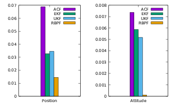
Bar plot in the High/High/High setting

Figure 1.14 is the plot of the tracking of the position (x, y, z) and attitute (r, i, j, k) in the low vicon precision, low accelerometer precision and low gyroscope precision setting for one of random trajectory.

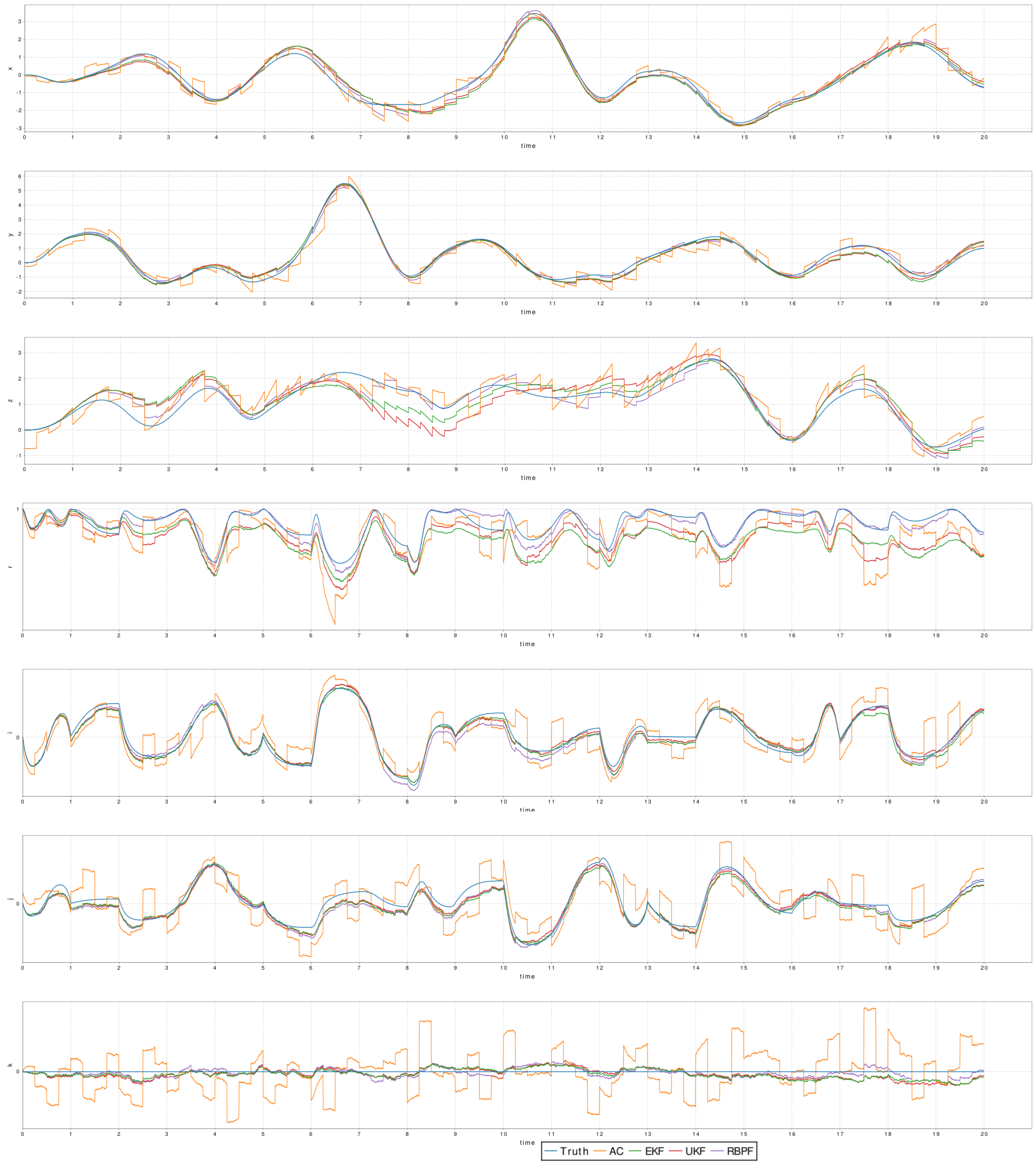
Plot of the tracking of the different filters

Conclusion

The Rao-Blackwellized Particle Filter developed is more accurate than the alternatives, mathematically sound and computationally feasible. When implemented on hardware, this filter can be executed in real time with sensors of high and asynchronous sampling rate. It could improve POSE estimation for all the existing drone and other robots. These improvements could unlock new abilities, potentials and increase the safeness of drone.

Part II

Continue here to read the section about scala-flow (II/IV)

References

[1] M. W. Mueller, M. Hehn, and R. D’Andrea, “A computationally efficient motion primitive for quadrocopter trajectory generation,” IEEE Transactions on Robotics, vol. 31, no. 6, pp. 1294–1310, 2015.
[2] F. L. Markley, Y. Cheng, J. L. Crassidis, and Y. Oshman, “Averaging quaternions,” Journal of Guidance, Control, and Dynamics, vol. 30, no. 4, pp. 1193–1197, 2007.
[3] K. Edgar, “A Quaternion-based Unscented Kalman Filter for Orientation Tracking.”.
[4] A. Doucet and A. M. Johansen, “A tutorial on particle filtering and smoothing: Fifteen years later,” Handbook of nonlinear filtering, vol. 12, nos. 656-704, p. 3, 2009.
[5] P. Vernaza and D. D. Lee, “Rao-Blackwellized particle filtering for 6-DOF estimation of attitude and position via GPS and inertial sensors,” in Robotics and Automation, 2006. ICRA 2006. Proceedings 2006 IEEE International Conference on, 2006, pp. 1571–1578.
-
The observation that the number of transistors in a dense integrated circuit doubles approximately every two years.↩
An embarrassingly parallel task is one where little or no effort is needed to separate the problem into a number of parallel tasks. This is often the case where there is little or no dependency or need for communication between those parallel tasks, or for results between them.↩
Gimbal lock is the loss of one degree of freedom in a three-dimensional, three-gimbal mechanism that occurs when the axes of two of the three gimbals are driven into a parallel configuration, “locking” the system into rotation in a degenerate two-dimensional space. ↩
The etymology for “Dead reckoning” comes from the mariners of the XVIIth century that used to calculate the position of the vessel with log book. The interpretation of “dead” is subject to debate. Some argue that it is a misspelling of “ded” as in “deduced”. Others argue that it should be read by its old meaning: absolute.↩